基于matlab小波去噪、小波包去噪、软硬阈值去噪、傅里叶去噪matlab相关代码
，直接替换数据就可以用。

小波去噪

% 读取或生成信号
load noisbloc; % 加载MATLAB自带的噪声信号
s = noisbloc;

% 执行小波分解
[C, L] = wavedec(s, 3, 'db4'); % 使用'db4'小波，分解到第3层

% 去噪处理（使用默认阈值）
[thr,sorh,keepapp] = ddencmp('den','wv',s); % 获取默认阈值等参数
clean = wdencmp('gbl',C,L,'db4',3,thr,sorh,keepapp); % 全局阈值去噪

% 绘制结果
subplot(2,1,1);
plot(s);
title('含噪声的信号');
subplot(2,1,2);
plot(clean);
title('去噪后的信号');

小波包去噪

% 读取或生成信号
load noisbloc;
s = noisbloc;

% 执行小波包分解
level = 3; % 分解层次
wpt = wpdec(s, level, 'db4'); % 使用'db4'小波

% 配置阈值
thrParams = wpthcoef('penalhi', wpt, 1.5); % 根据需要调整阈值

% 去噪处理
clean = wprcoef(thrParams);

% 绘制结果
subplot(2,1,1);
plot(s);
title('含噪声的信号');
subplot(2,1,2);
plot(clean);
title('去噪后的信号');

软硬阈值去噪

% 生成或加载信号
x = linspace(0,1,1000);
original_signal = sin(2*pi*60*x) + sin(2*pi*200*x); % 创建一个测试信号
noisy_signal = original_signal + 0.5*randn(size(original_signal)); % 添加噪声

% 进行小波变换并选择阈值
[C, L] = wavedec(noisy_signal, 5, 'sym8');
thr = sqrt(2*log(length(noisy_signal))); % 通用阈值公式

% 应用软阈值
soft_denoised = wthresh(C, 's', thr);
[~, ~, ~, ~, ~, soft_reconstructed] = waverec([soft_denoised, zeros(1,length(C)-length(soft_denoised))], L, 'sym8');

% 应用硬阈值
hard_denoised = wthresh(C, 'h', thr);
[~, ~, ~, ~, ~, hard_reconstructed] = waverec([hard_denoised, zeros(1,length(C)-length(hard_denoised))], L, 'sym8');

% 绘制结果
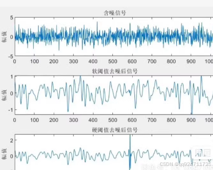
subplot(3,1,1);
plot(noisy_signal);
title('含噪声的信号');
subplot(3,1,2);
plot(soft_reconstructed);
title('软阈值去噪后的信号');
subplot(3,1,3);
plot(hard_reconstructed);
title('硬阈值去噪后的信号');

傅里叶去噪

% 生成或加载信号
fs = 1000; % 采样频率
t = 0:1/fs:1-1/fs; % 时间向量
x = cos(2*pi*50*t) + cos(2*pi*120*t); % 创建一个测试信号
y = x + 2*randn(size(t)); % 添加噪声

% 进行傅里叶变换
Y = fft(y);

% 创建滤波器
f = fs*(0:(length(Y)/2))/length(Y); % 频率向量
desired_frequencies = (f >= 45 & f <= 55) | (f >= 115 & f <= 125); % 指定保留的频率范围
filtered_Y = Y .* [desired_frequencies, fliplr(desired_frequencies(2:end-1 or length(Y) == 1))]; % 应用滤波器

% 反傅里叶变换
clean_signal = ifft(filtered_Y);

% 绘制结果
subplot(2,1,1);
plot(t,y);
title('含噪声的信号');
xlabel('时间 (秒)');
ylabel('幅值');
subplot(2,1,2);
plot(t,real(clean_signal));
title('傅里叶去噪后的信号');
xlabel('时间 (秒)');
ylabel('幅值');

请注意，以上代码仅为示例，具体应用时可能需要根据你的数据和需求进行适当的调整。此外，在实际操作中，选择合适的小波基函数、分解层数、阈值策略等都是影响去噪效果的重要因素。

如何使用MATLAB进行小波包去噪。这个例子假设你已经有了一个包含噪声的信号，并且你想通过小波包分解和阈值处理来去除噪声。

小波包去噪

% 生成或加载含噪声的信号
fs = 1000; % 采样频率
t = 0:1/fs:1-1/fs; % 时间向量
x = cos(2*pi*50*t) + cos(2*pi*120*t); % 创建一个测试信号
noisy_signal = x + 2*randn(size(t)); % 添加噪声

% 绘制原始信号
figure;
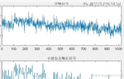
subplot(2,1,1);
plot(t, noisy_signal);
title('含噪声的信号');
xlabel('时间 (秒)');
ylabel('幅值');

% 执行小波包分解
level = 3; % 分解层次
wname = 'db4'; % 小波基函数
wpdec_tree = wpdec(noisy_signal, level, wname);

% 配置阈值
thrParams = wpthcoef('penalhi', wpdec_tree, 1.5); % 根据需要调整阈值

% 去噪处理
clean_signal = wprcoef(thrParams);

% 绘制去噪后的信号
subplot(2,1,2);
plot(t, clean_signal);
title('小波包去噪后的信号');
xlabel('时间 (秒)');
ylabel('幅值');

解释

1. 生成或加载信号：

   • fs 是采样频率。
   • t 是时间向量。
   • x 是原始信号（这里使用了两个正弦波）。
   • noisy_signal 是添加了高斯噪声的信号。

2. 绘制原始信号：

   • 使用 subplot 和 plot 函数绘制原始信号。

3. 执行小波包分解：

   • level 是分解层次。
   • wname 是小波基函数（这里使用的是 db4）。
   • wpdec 函数用于进行小波包分解。

4. 配置阈值：

   • wpthcoef 函数用于设置阈值参数。

5. 去噪处理：

   • wprcoef 函数用于重构信号并应用阈值处理。

6. 绘制去噪后的信号：

   • 使用 subplot 和 plot 函数绘制去噪后的信号。

软硬阈值去噪

如果你还想尝试软阈值和硬阈值去噪，可以参考以下代码：

% 小波分解
[C, L] = wavedec(noisy_signal, 3, 'db4'); % 使用'db4'小波，分解到第3层

% 获取默认阈值等参数
[thr, sorh, keepapp] = ddencmp('den', 'wv', noisy_signal);

% 应用软阈值
soft_denoised = wdencmp('gbl', C, L, 'db4', 3, thr, 's');

% 应用硬阈值
hard_denoised = wdencmp('gbl', C, L, 'db4', 3, thr, 'h');

% 绘制结果
figure;
subplot(3,1,1);
plot(t, noisy_signal);
title('含噪声的信号');
subplot(3,1,2);
plot(t, soft_denoised);
title('软阈值去噪后的信号');
subplot(3,1,3);
plot(t, hard_denoised);
title('硬阈值去噪后的信号');

傅里叶去噪

% 进行傅里叶变换
Y = fft(noisy_signal);

% 创建滤波器
f = fs*(0:(length(Y)/2))/length(Y); % 频率向量
desired_frequencies = (f >= 45 & f <= 55) | (f >= 115 & f <= 125); % 指定保留的频率范围
filtered_Y = Y .* [desired_frequencies, fliplr(desired_frequencies(2:end-1))]; % 应用滤波器

% 反傅里叶变换
clean_signal_fft = ifft(filtered_Y);

% 绘制结果
figure;
subplot(2,1,1);
plot(t, noisy_signal);
title('含噪声的信号');
xlabel('时间 (秒)');
ylabel('幅值');
subplot(2,1,2);
plot(t, real(clean_signal_fft));
title('傅里叶去噪后的信号');
xlabel('时间 (秒)');
ylabel('幅值');

这些代码片段可以帮助你理解和实现小波包去噪、软硬阈值去噪以及傅里叶去噪。请根据你的具体需求进行调整。