目录
目录
摘要
一种基于层次分析法的大数据排序方法。层次分析法(AHP)是分析决策中常用的方法,但是其使用数据量有所限制,在我们想将大量数据进行排序处理的时候,层次分析法往往显得无力。本文主要介绍了将层次分析法推广的大量数据的方法,使得层次分析法可以在大量数据中,进行排序。
一、灵感来源以及应用背景(一些废话)
各位大佬早上中午晚上好。
这个是我在做今年华数杯的时候,突然想到了一个解决方案,方案可能不完整,可能有些我没有发现的小的逻辑漏洞。但我感觉大体上是没有问题的,欢迎各路大佬批评指正!
简单说一下华数杯第二问的背景吧,就是给了我们346个城市(题目原本要求比较的城市是比346要多的,但是官方给的数据集也不完整,我自己去网上买的数据集剔除了几个城市,就只剩下346个城市),然后要我们给这346个城市按照城市规模、环境保护、人文底蕴、交通便利、气候、美食这6个因素来给城市排序。讲道理这个应该是可以用层次分析法来解决,但是由于这个数据量太大了,层次分析法没法比较346个城市,所以就有了这篇文章。
关于层次分析法在我前面的文章有提到,大家不太熟悉的可以去看一下。层次分析法(AHP)(案例+Python实现)_层次分析法ahp矩阵文件-CSDN博客
二、思想和解决过程
其实我的做法(或者思想)很简单,就是“两两比较、好的留下”。但是具体实现还是没有这么简单。下面直接放流程图,后面会解释。

按照上述流程图,首先导入346个城市数据,然后每5个为一组(向上取整),这样我们就可以得到70组,70组每为5个城市,构建这5个城市的判断矩阵,然后对这5个城市进行层次分析法,就可以筛选出每组最好的城市,这样我们就可以筛选出70个最好的城市(因为有70组)。我们把这70组放到一个集合里,我们就把这个集合叫做最好城市集合,剩下的276个城市放到另一个城市集合中,我们就把这个集合叫做次好城市集合。接下来我们判断次好城市集合中的城市数量是否大于5个,如果大于5个,那么就在重复分组、建立判断矩阵、层次分析、筛选每组最好城市的操作。直到次好城市集合里的集合数量小于5个,这个时候我们对这些城市(小于5个)进行层次分析法,得到他们的排名顺序,放入栈中,此时栈更新,我们让最好城市集合里的数据再重复分组、建立判断矩阵、层次分析、筛选每组最好城市的操作。最好城市集合里的城市数量小于5,此时我们再对这些城市进行层次分析法,进行排序,最后放入栈中,此时所有的城市数据处理完毕,且排好了序,此时栈为城市排名降序排序。即最好的在栈顶(最上面)。
有几点需要说明:
- 上述流程图中的清空xx集合只是清空集合,为后续操作腾出空间,并不是删除数据!!!数据还是正常在流程中运行!!!
- 栈是一种先进后出的数据结构,如果你不了解可以去简单学一下,这东西很简单。
- 如果你还是看不明白的话可以看看接下来的伪代码和举例说明
三、举例说明
由于346个城市数据量还是太大了点,所以我以简单的20个城市作为例子进行说明。
假设我们有20个城市需要进行比较:
- step1:对这20个城市进行分组,每5个为一组,分为4组。
- step2:每组内进行层次分析法,选出每组最好的城市,这样就筛选出最好的4个城市。
- step3:把这4个城市放到一个集合里,就叫最好城市集合,剩下的16个城市放到另一个集合里,就叫次好城市集合。
- step4:对剩下的16个城市再进行分组,5个为一组,分4组。
- step5:每组内部进行层次分析比较,得到最好的城市,此时筛选出4个最好城市。
- step6:将这3个城市加入到最好城市集合里,也就是4+4=8个城市,此时次好城市集合还剩下16-4=12个城市。
- step7:对这12个城市进行分组,5个为一组,分3组(向上取整)。
- step8:重复step5、step6,此时,次好城市集合里还剩下12-3=9个城市。最好城市集合有8+3=11个城市。
- step9:对这9个城市分组,5个为一组,分为2组。
- step10:重复step5、step6,此时,次好城市集合里还剩下9-2=7个城市。最好城市集合有11+2=13个城市。
- step11:对这7个城市分组,5个为一组,分为2组。
- step12:重复step5、step6,此时,次好城市集合里还剩下7-2=5个城市。最好城市集合有13+2=15个城市。
- step13:此时次好城市集合里的城市数量已经小于5,我们对这5个城市利用层次分析法进行排序。
- step14:将排好序的5个城市放入栈中,此时栈中有5个排好序的数据。
- step15:对最好城市集合了的15个城市分组,5个为一组,分3组。
- step16:重复step2,选出最好的3个城市,将着3个城市放入一个新的最好城市集合,此时最好城市集合里有3个城市,剩下15-3=12个城市仿佛一个新的次好城市集合,此时有12个城市。(接下是重复,过程会些简略,我会算完,如过你已经懂了可以不用看了)
- step17:12个分组,分3组。层次分析法后,最好城市集合里有3+3=6个城市,次好城市集合里有12-3=9个城市。
- step18:重复step17,9分两组,层次分析法后,最好城市集合里有6+2=8个城市,次好城市集合里有9-2=7个城市。
- step19:重复step17,7分两组,层次分析法后,最好城市集合里有8+2=10个城市,次好城市集合里有7-2=5个城市。
- step20:5个城市进行层次分析排序,放入栈中,此时栈中有10个降序排列的城市。
- step21:剩下10个城市未排序,10分2组,层次分析后,最好城市集合有2个,次好城市集合里有10-2=8个城市。
- step22:8分2组,层次分析后,最好城市集合有2+2=4个,次好城市集合里有8-2=6个城市。
- step23:6分2组,层次分析后,最好城市集合有4+2=6个,次好城市集合里有6-2=4个城市。
- step24:4小于5,对这4个城市进行层次分析,放入栈中,此时栈有14个城市。
- step25:剩下6个城市未排序,6分2组,最好城市集合有2个,次好城市集合里有6-2=4个城市。
- step26:4小于5,对这4个城市进行层次分析,放入栈中,此时栈有18个城市。
- step27:剩下2个城市未排序,2小于5,对这两个城市进行层次分析,放入栈中,此时栈20个城市,所有城市处理完毕。
四、伪代码
伪代码是我实现该算法的思路,大家可以参考着看一下,总的来说我并没有创建这么多个集合,我采用的是删除的方式,就是如果你是最好城市,你就剔除掉次好城市中,然后一次筛选完毕后,我们得到小于5的坏城市,在把这5个坏城市从最好城市列表中剔除。这就是我代码的大体思路,可能不是很清楚,但是代码这个东西,每个人的思路不一样,你也可以自己去实现这个算法,我表达能力有限,没法很好的讲代码,就放了段伪代码共大家观赏。欢迎大佬给出更好的解法。
需要注意的是,当只有一个城市的时候,不适合层次分析法,需要单独讨论,大家编写程序的时候需要注意。
"""
伪代码
"""

best_citys = all_data
second_best_citys = best_city
Stack = None

while len(best_citys) > 5:
    while len(second_best_citys) > 5:
        city_groups = second_best_citys divide into groups
        for group in city_groups:
            group by AHP
            find best city in group
            second_best_city delete best city
    city_list = second_best_citys by AHP
    city_list push Stack
    best_citys delete city_list
    second_best_citys = best_citys
city_list = best_citys by AHP
city_list push Stack
这里
五、实战以及数据集效果
接下来看看这个算法在华数杯C题数据集上的表现。
首先就是这个数据集,比较长,我就放一部分。大家看看就好。这个数据集是用来确定我们的决策矩阵用的。
| 来源城市 | AQI | 绿化覆盖率 (%) | 废水处理率 (%) | 废气处理率 (%) | 垃圾分类处理率 (%) | 历史遗迹数量 | 博物馆数量 | 文化活动频次 | 文化设施数量 | 公共交通覆盖率 (%) | 线路密度 (km/km²) | 高速公路里程 (km) | 机场航班数量 | 年平均气温 (℃) | 年降水量 (mm) | 适宜旅游天数 | 空气湿度 (%) | 餐馆数量 | 特色美食数量 | 美食活动频次 |
| 阿坝 | 50 | 36 | 88 | 85 | 73 | 14 | 5 | 20 | 16 | 75 | 1.3 | 280 | 42 | 13 | 800 | 220 | 57 | 160 | 32 | 14 |
| 阿克苏 | 45 | 34 | 86 | 83 | 70 | 12 | 4 | 22 | 15 | 75 | 1.2 | 270 | 40 | 12 | 700 | 220 | 55 | 160 | 30 | 14 |
| 阿拉尔 | 49 | 33 | 87 | 84 | 72 | 13 | 5 | 22 | 18 | 76 | 1.4 | 280 | 42 | 11 | 650 | 230 | 57 | 170 | 35 | 15 |
| 阿勒泰 | 50 | 36 | 88 | 85 | 73 | 14 | 5 | 20 | 16 | 75 | 1.3 | 280 | 42 | 13 | 800 | 220 | 57 | 160 | 32 | 14 |
| 阿里 | 48 | 37 | 89 | 86 | 74 | 12 | 5 | 22 | 17 | 78 | 1.4 | 290 | 44 | 16 | 900 | 240 | 58 | 170 | 35 | 15 |
| 安康 | 46 | 35 | 87 | 84 | 72 | 13 | 5 | 23 | 17 | 77 | 1.5 | 295 | 46 | 14 | 850 | 230 | 60 | 175 | 38 | 16 |
针对这个数据集,我们需要讲他变为城市规模、环境保护、人文底蕴、交通便利、气候、美食这6个因素,非常不幸的是,这个数据集里没有城市规模,所以我们只好忍痛割掉城市规模这个因素,剩下环境保护、人文底蕴、交通便利、气候、美食这5个因素。
我的做法也很简单,首先按列归一化
| 城市 | AQI | 绿化覆盖率 (%) | 废水处理率 (%) | 废气处理率 (%) | 垃圾分类处理率 (%) | 历史遗迹数量 | 博物馆数量 | 文化活动频次 | 文化设施数量 | 公共交通覆盖率 (%) | 线路密度 (km/km²) | 高速公路里程 (km) | 机场航班数量 | 年平均气温 (℃) | 年降水量 (mm) | 适宜旅游天数 | 空气湿度 (%) | 餐馆数量 | 特色美食数量 | 美食活动频次 |
| 阿坝 | 0.31068 | 0.6 | 0.428571 | 0.555556 | 0.3 | 0.266667 | 0.166667 | 0.25 | 0.222222 | 0.6 | 0.111111 | 0.533333 | 0.55 | 0.416667 | 0.541667 | 0.4 | 0.35 | 0.3 | 0.125 | 0.266667 |
| 阿克苏 | 0.262136 | 0.4 | 0.142857 | 0.333333 | 0 | 0.133333 | 0 | 0.35 | 0.166667 | 0.6 | 0 | 0.466667 | 0.5 | 0.333333 | 0.458333 | 0.4 | 0.25 | 0.3 | 0.0625 | 0.266667 |
| 阿拉尔 | 0.300971 | 0.3 | 0.285714 | 0.444444 | 0.2 | 0.2 | 0.166667 | 0.35 | 0.333333 | 0.64 | 0.222222 | 0.533333 | 0.55 | 0.25 | 0.416667 | 0.5 | 0.35 | 0.35 | 0.21875 | 0.333333 |
| 阿勒泰 | 0.31068 | 0.6 | 0.428571 | 0.555556 | 0.3 | 0.266667 | 0.166667 | 0.25 | 0.222222 | 0.6 | 0.111111 | 0.533333 | 0.55 | 0.416667 | 0.541667 | 0.4 | 0.35 | 0.3 | 0.125 | 0.266667 |
| 阿里 | 0.291262 | 0.7 | 0.571429 | 0.666667 | 0.4 | 0.133333 | 0.166667 | 0.35 | 0.277778 | 0.72 | 0.222222 | 0.6 | 0.6 | 0.666667 | 0.625 | 0.6 | 0.4 | 0.35 | 0.21875 | 0.333333 |
然后和环境保护相关指标,直接相加,例如阿坝的环境保护得分为0.31068+0.6+0.428571+0.555556+0.3+0.266667=2.461474,人文底蕴这些同理。然后在按列归一化。得到下列数据。
| 城市 | 环境保护 | 人文底蕴 | 交通便利 | 气候 | 美食 |
| 阿坝 | 0.53165 | 0.226389 | 0.461429 | 0.4038 | 0.214184 |
| 阿克苏 | 0.257551 | 0.1625 | 0.402857 | 0.327791 | 0.192908 |
| 阿拉尔 | 0.359462 | 0.2625 | 0.500286 | 0.349169 | 0.285816 |
| 阿勒泰 | 0.53165 | 0.226389 | 0.461429 | 0.4038 | 0.214184 |
| 阿里 | 0.644392 | 0.231944 | 0.550857 | 0.570071 | 0.285816 |
然后层次分析法需要指标定量化,这个我也非常暴力。直接看表吧,


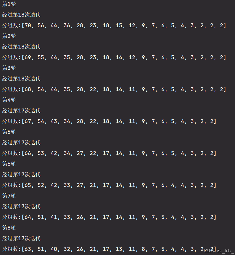
看看运行结果:
这事前8轮运行结果
这是后8轮运行结果

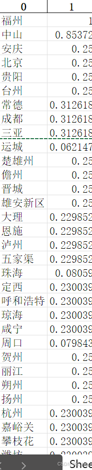
我们看看最后程序写入的Excle表格,这里给出前十排名,这里分数是乱的,算法特点,正常的,但排名是正确的。
| 0 | 1 |
| 福州 | 1 |
| 中山 | 0.85372 |
| 安庆 | 0.25 |
| 北京 | 0.25 |
| 贵阳 | 0.25 |
| 台州 | 0.25 |
| 常德 | 0.312618 |
| 成都 | 0.312618 |
| 三亚 | 0.312618 |
写入的excle表格就长这样。
六、程序源码
ps:这个代码不是傻瓜代码,不能复制粘贴下来直接跑!!!这个是我参加比赛时跑的代码,很多数据和路径都是我自己的,里面也有很多画图的代码和我保存临时文件的代码,所以你要是想用可能需要魔改一下,至于为什么不写一份傻瓜式代码,因为我懒【狗头】。你若是想用但又看不懂我代码可以私信或者评论问我,(毕竟我代码确实写得有点烂)我看到了都会回的。想要数据集的也可以私信和评论区找我要,我打包给你。【狗头】
"""
@ S_Iris_
AHP(big_data)
仅供学习交流使用
"""

import pandas as pd
import os
import math
import random
import numpy as np
import matplotlib.pyplot as plt
plt.rcParams['font.sans-serif'] = ['SimHei']    # 用来正常显示中文标签
plt.rcParams['axes.unicode_minus'] = False    # 用来显示负号

def score(_data_, left, right):
    data = _data_.copy()
    if right == 0:
        block_data = data.iloc[:, left:]
    else:
        block_data = data.iloc[:, left:right]
    the_score = block_data.iloc[:, 0]
    for i in range(1, block_data.shape[1]):
        the_score = the_score + block_data.iloc[:, i]

    return block_data, the_score


# 分组
def divide_into_groups(_data_, n=5):
    data = np.zeros_like(_data_)
    data[:] = _data_[:]
    groups = []
    shape = data.shape
    count = int(shape[0] / n)
    if shape[0] % n != 0:
        count += 1
    for i in range(0, count):
        if i != (count-1):
            group = data[i*5:i*5+5, :]
            groups.append(group)
        else:
            group = data[i*5:, :]
            groups.append(group)
    return groups, count


# AHP
def AHP(evaluate):
    # RI表
    RI_sheet = {'1': 0, '2': 0, '3': 0.52, '4': 0.89, '5': 1.12, '6': 1.26, '7': 1.36,
                '8': 1.41, '9': 1.46, '10': 1.49, '11': 1.52, '12': 1.54, '13': 1.56,
                '14': 1.58, '15': 1.59}

    data_characteristic = []
    uni_data = []
    data_omega = []

    # 归一化
    for i in range(0, len(evaluate)):
        arr = evaluate[i][:, 1:]
        arr = arr.astype(float)
        nui_arr = np.zeros_like(arr)
        nui_arr[:] = arr[:]
        nui_arr = nui_arr.astype(np.float32)
        shape = nui_arr.shape
        sum = nui_arr.sum(axis=0)
        for n in range(0, shape[1]):
            nui_arr[:, n] = nui_arr[:, n] / sum[n]
        omega = nui_arr.sum(axis=1) / shape[1]
        data_omega.append(omega)

    evaluate_list = evaluate[-1][:, 0]
    lo_name = evaluate[1][:, 0]
    Z = np.zeros((len(evaluate_list), (len(lo_name)+1)), dtype=float)
    Z[:, 0] = data_omega[-1]
    for i in range(0, len(evaluate_list)):
        Z[i, 1:] = data_omega[i]

    shape = Z.shape
    sum = []
    weight = data_omega[-1]
    for i in range(1, shape[1]):
        sum1 = np.dot(weight, Z[:, i])
        sum.append(sum1)

    decision = np.argmax(sum)
    decision = lo_name[decision]

    result = np.array(sum)
    result = np.vstack((lo_name, result))
    result = result.T

    result = pd.DataFrame(result)
    result = result.sort_values(axis=0, ascending=False, by=1)

    return decision, result


def judge(x):
    v = 1
    flag = 1
    if x < 0:
        flag = 0
    x = abs(x)
    if x > 0.7:
        v = 9
    elif x < 0.7 and x > 0.6:
        v = 8
    elif x > 0.5 and x < 0.6:
        v = 7
    elif x > 0.4 and x < 0.5:
        v = 6
    elif x > 0.3 and x < 0.4:
        v = 5
    elif x > 0.2 and x < 0.3:
        v = 4
    elif x > 0.1 and x < 0.2:
        v = 3
    elif x < 0.1 and x > 0.05:
        v = 2
    elif x < 0.05:
        v = 1
    if flag == 0:
        v = float(1/v)

    return v


def last_judgment_matrix(_groups_):
    arr = np.zeros_like(_groups_)
    arr[:] = _groups_[:]
    city_name = arr[:, 0]
    value = arr[:, 1:]
    value = value.astype(float)
    shape = arr.shape
    group = []
    for j in range(0, shape[1]-1):
        norm = np.zeros((shape[0], shape[0]))
        # norm[:, 0] = city_name[:]
        for n in range(0, shape[0]):
            for k in range(0, shape[0]):
                x = value[n, j] - value[k, j]
                v = judge(x)
                norm[n, k] = v
        city_name = city_name.reshape(shape[0], 1)
        norm = np.hstack((city_name, norm))
        group.append(norm)
    return group


def judgment_matrix(_groups_):
    groups = []
    groups[:] = _groups_[:]
    count = len(groups)
    evaluates = []
    for i in range(0, count):
        arr = groups[i]
        city_name = arr[:, 0]
        value = arr[:, 1:]
        value = value.astype(float)
        shape = arr.shape
        group = []
        for j in range(0, shape[1]-1):
            norm = np.zeros((shape[0], shape[0]))
            # norm[:, 0] = city_name
            for n in range(0, shape[0]):
                for k in range(0, shape[0]):
                    x = value[n, j] - value[k, j]
                    v = judge(x)
                    norm[n, k] = v
            city_name = city_name.reshape(shape[0], 1)
            norm = np.hstack((city_name, norm))
            group.append(norm)
        evaluates.append(group)
    return evaluates


def figure(js, nn):
    for i in range(0, len(js)):
        fig1 = plt.figure(1)
        fig1.supxlabel('迭代次数')
        fig1.supylabel('分组数')
        fig1.suptitle('第{}轮收敛情况'.format(i))
        x = [i+1 for i in range(js[i])]
        y = nn[i]
        fig1 = plt.scatter(x, y)
        plt.savefig(r'.\2024huashu\c\2\figure(散点)\第{}轮次收敛情况.jpg'.format(i))
        plt.close()
    # 子图绘制
    a, b = 3, 3
    fig = plt.figure(figsize=(12, 6), dpi=100, facecolor='w')
    fig.suptitle('轮次内部收敛情况')
    for i in range(0, 9):
        ax = plt.subplot(a, b, i + 1)
        ax.tick_params(axis='both', colors='black', direction='out', labelsize=15, width=1, length=1, pad=5)
        x = [i+1 for i in range(js[-i])]
        y = nn[-i]
        ax.scatter(x, y)
        if math.ceil((i + 1) / b) != a:
            plt.xticks([0, 20])
        if i % b != 0:
            plt.yticks([0, 70])
    # plt.savefig('后9轮次内部收敛情况(散点).jpg')
    plt.close()

def main():
    work_path = os.getcwd()
    path = r'\subjectC\BZD-最终版数据集无水印[更正版].xlsx'
    data = pd.read_excel(path)
    # 剔除第一列(城市名称)
    new_data = data.iloc[:, 1:]
    city_names = data.iloc[:, 0]
    # 归一化处理
    nl_data = (new_data - new_data.min()) / (new_data.max() - new_data.min())
    nl_data_city = nl_data.copy()
    nl_data_city.insert(loc=0, column='城市', value=data.iloc[:, 0])
    # nl_data_city.to_excel('nl_data.xlsx', index=False) # 保存文件

    # 环境保护分块
    env_prot_data, env_score = score(nl_data, 0, 5)
    # 人文底蕴分块
    cultural_data, cultural_score = score(nl_data, 5, 9)
    # 交通便利分块
    traffic_data, traffic_score = score(nl_data, 9, 13)
    # 气候分块
    climate_data, climate_score = score(nl_data, 13, 17)
    # 美食分块
    food_data, food_score = score(nl_data, 17, 0)

    # 因素得分
    temp_data = [env_score, cultural_score, traffic_score, climate_score, food_score]
    columns = ['环境保护', '人文底蕴', '交通便利', '气候', '美食']
    point_score = pd.DataFrame(temp_data, columns)
    point_score = point_score.transpose()
    nl_score = (point_score - point_score.min()) / (point_score.max() - point_score.min())
    nl_score.insert(loc=0, column='城市', value=city_names)
    # nl_score.to_excel('nl_score.xlsx', index=False) # 保存文件

    evaluate = np.array([['环境保护', 1.00, 1.00, 1.00, 1.00, 1.00],
                         ['人文底蕴', 1.00, 1.00, 1.00, 1.00, 1.00],
                         ['交通便利', 1.00, 1.00, 1.00, 1.00, 1.00],
                         ['气候', 1.00, 1.00, 1.00, 1.00, 1.00],
                         ['美食', 1.00, 1.00, 1.00, 1.00, 1.00]])

    win_data = nl_score.values
    no_data = nl_score.values
    shape = nl_score.shape
    loss_data = np.zeros((1, 2))
    nnn = []
    js = []
    i_s = []
    i = 0
    while len(win_data) > 5:
        i += 1
        i_s.append(i)
        print("第{}轮".format(i))
        j = 0
        nn = []
        while len(no_data) > 5:
            j += 1
            groups, count = divide_into_groups(no_data, n=5)
            print("\r经过第{}次迭代".format(j), end=" ")
            nn.append(count)
            # 构建判断矩阵
            evaluates = judgment_matrix(groups)
            for k in range(0, count):
                # print(r"{}".format(i), end=" ")
                group = evaluates[k]
                a = group[0].shape[0]
                if a == 1:
                    decision = group[0][:, 0]
                else:
                    group.append(evaluate)
                    decision, result = AHP(group)
                index = np.where(no_data[:, 0] == decision)
                no_data = np.delete(no_data, index, axis=0)
        nnn.append(nn)
        js.append(j)
        print("")
        print("分组数:{}".format(nn))
        # 降序排列
        if len(no_data) == 1:
            result = no_data[:, 0:2]
        else:
            group = last_judgment_matrix(no_data)
            decision, result = AHP(group)
            result = result.values
        loss_data = np.vstack((result, loss_data))
        n = result.shape[0]
        for k in range(0, n):
            name = result[k, 0]
            index = np.where(win_data[:, 0] == name)
            win_data = np.delete(win_data, index, axis=0)
        no_data = np.zeros_like(win_data)
        no_data[:] = win_data[:]
    fig = plt.figure(1)
    fig.supxlabel('训练轮次')
    fig.supylabel('迭代次数')
    fig.suptitle('整体收敛情况')
    fig = plt.scatter(i_s, js)
    # plt.savefig(r'.\2024huashu\c\2\整体收敛(散点).jpg')
    # plt.show()
    plt.close()

    # figure(js, nnn)

    best_city = win_data[:, 0:2]
    loss_data = np.vstack((best_city, loss_data))
    result = pd.DataFrame(loss_data)
    # result.to_excel('result.xlsx', index=False)


if __name__ == "__main__":
    main()
七、评价
说几点,我觉得算法可以改进和优化的地方,还有算法迁移的难点,和一些缺点(说些不敢写进论文里的东西【狗头】)
缺点:
- 我这里的层次分析法没有加入一致性检验,因为我在debug的时候,一致性检验会出问题,就把这东西删了,但后来发现不是一致性检验的问题,是其他地方的bug,但当时赶时间,就懒得加了。不过按照我的建立决策矩阵的方式,我觉得不应该会出现不通过一致性检验的地方。
改进和优化:
- 我采用的其实算是一种暴力算法,346个数据算起来其实还蛮快了,5-6秒就算完了,但是如果更大的数据量我感觉可能会算更久,但我也没有测试过,各位大佬可以提些加速方法。
- 我这个是在AHP的方案层有大量数据,但没有考虑在指标层出现大量数据的情况,各位大佬有兴趣可以拿去改改。
算法迁移难点:
- 算法迁移的难点其实在于决策矩阵的建立,需要批量化建立决策矩阵的方法,这个东西目前来看,每个数据的建立方法不同,不好统一处理,这是我感觉的一个迁移难点。
好了,感谢你看到这里,送你一只折枝,祝你天天开心!