1概括
声明:文章里面一些原理图片来自《Attention Is All You Need》如有侵权请及时联系,本文作为笔者自己学习时的学习记录,若有侵权请及时联系
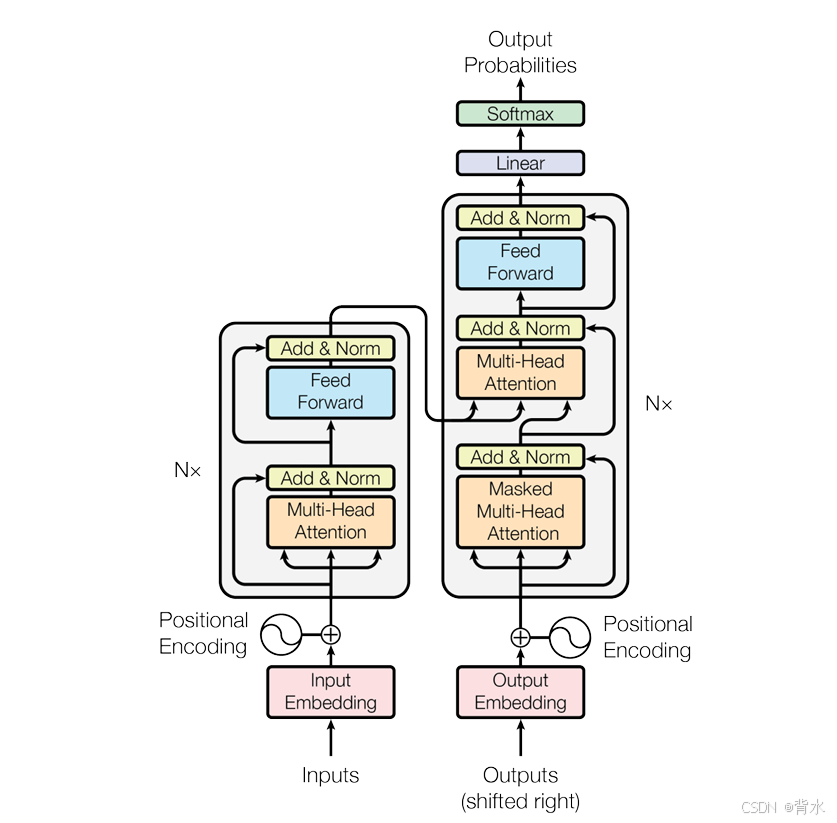
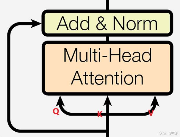
首先介绍Transformer由哪些部分组成。
1.1整体架构
上图来自《Attention Is All You Need》。
2.详细解释
2.1 输入部分
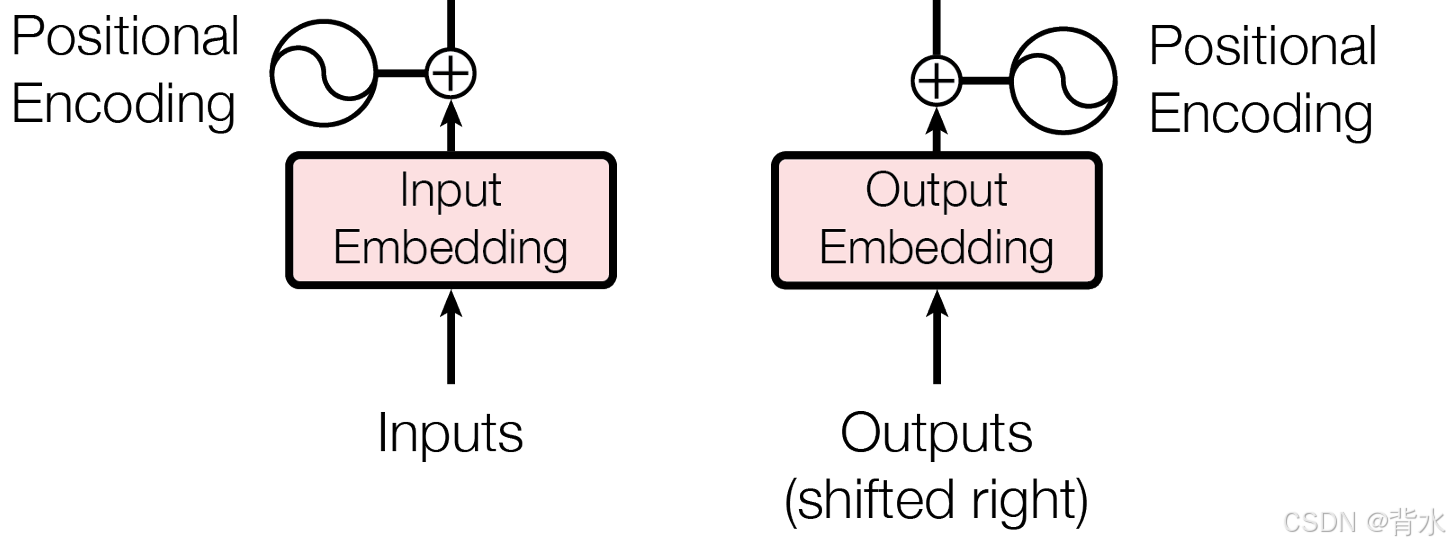
源文本嵌入层及其位置编码器目标文本嵌入层及其位置编码器
2.1.1词嵌入层代码
无论是源文本嵌入层还是目标文本嵌入层都属于词嵌入层。词嵌入曾仅是简单的讲输入转化为具体的张量,最后由于需要与位置编码器的量纲保持一致,需要乘一个参数。
class Embeddings(nn.Module):
    def __init__(self, dim_model, vocabulary):
        """
        :param dim_model: 词嵌入的尺寸(每个单词需要多少维表示)
        :param vocabulary: 总共的单词的数量
        """
        super(Embeddings, self).__init__()
        self.dim_model = dim_model
        self.vocabulary = vocabulary
        self.embedding = nn.Embedding(num_embeddings=vocabulary, embedding_dim=dim_model)
    def forward(self, x):
        # 词向量与位置编码特征向量相加,乘一个数以保持量纲一直
        x = self.embedding(x) * math.sqrt(self.dim_model)
        return x
2.1.2位置编码器
位置编码的主要作用是:
- 为模型提供位置信息:让模型知道每个词在序列中的具体位置
- 区分相同词在不同位置的意义:例如,句子“我和同学一起听和光同尘”中,第一个“和”是连词,第二个“和”是介词,位置编码可以帮助模型区分它们
- 保持序列的顺序性:位置编码确保模型能够正确处理序列中词的顺序关系。
2.1.2.1 位置编码的数学原理
位置编码通过正弦和余弦函数生成,公式如下:
P
E
(
p
o
s
,
2
i
)
=
sin
(
p
o
s
1000
0
2
i
d
model
)
PE_{(pos, 2i)} = \sin\left(\frac{pos}{10000^{\frac{2i}{d_{\text{model}}}}}\right)
PE(pos,2i)=sin(10000dmodel2ipos)
P
E
(
p
o
s
,
2
i
+
1
)
=
cos
(
p
o
s
1000
0
2
i
d
model
)
PE_{(pos, 2i+1)} = \cos\left(\frac{pos}{10000^{\frac{2i}{d_{\text{model}}}}}\right)
PE(pos,2i+1)=cos(10000dmodel2ipos)
其中:
- p o s pos pos:词在序列中的位置(从0开始)。
- i i i:维度索引(从0到 d model 2 − 1 \frac{d_{\text{model}}}{2} - 1 2dmodel−1)。
- d model d_{\text{model}} dmodel:模型的维度(通常是512或768)。
公式的直观解释
- 正弦和余弦交替使用:偶数维度用正弦函数,奇数维度用余弦函数。这种交替设计使得位置编码能够捕捉到不同频率的变化。
- 频率递减:随着维度
i
i
i的增加,
频率逐渐降低(因为分母 1000 0 2 i d model 10000^{\frac{2i}{d_{\text{model}}}} 10000dmodel2i逐渐增大)。低频编码捕捉全局位置信息,高频编码捕捉局部位置信息。 - 唯一性:每个位置的位置编码是唯一的,即使是相同的词,在不同位置也会有不同的编码。
具体例子:句子“我和同学一起听和光同尘”
假设句子是“我和同学一起听和光同尘”,分词结果为:
['我', '和', '同学', '一起', '听', '和', '光同尘']
序列长度为7,假设模型维度 d model = 4 d_{\text{model}} = 4 dmodel=4。
- 步骤1:生成位置编码
根据公式,计算每个位置的位置编码。以位置2(第一个“和”)和位置6(第二个“和”)为例:
位置2的编码
P
E
(
2
,
0
)
=
sin
(
2
1000
0
0
4
)
=
sin
(
2
)
≈
0.9093
PE_{(2, 0)} = \sin\left(\frac{2}{10000^{\frac{0}{4}}}\right) = \sin(2) \approx 0.9093
PE(2,0)=sin(10000402)=sin(2)≈0.9093
P
E
(
2
,
1
)
=
cos
(
2
1000
0
0
4
)
=
cos
(
2
)
≈
−
0.4161
PE_{(2, 1)} = \cos\left(\frac{2}{10000^{\frac{0}{4}}}\right) = \cos(2) \approx -0.4161
PE(2,1)=cos(10000402)=cos(2)≈−0.4161
P
E
(
2
,
2
)
=
sin
(
2
1000
0
2
4
)
=
sin
(
0.0002
)
≈
0.0002
PE_{(2, 2)} = \sin\left(\frac{2}{10000^{\frac{2}{4}}}\right) = \sin(0.0002) \approx 0.0002
PE(2,2)=sin(10000422)=sin(0.0002)≈0.0002
P
E
(
2
,
3
)
=
cos
(
2
1000
0
2
4
)
=
cos
(
0.0002
)
≈
1
PE_{(2, 3)} = \cos\left(\frac{2}{10000^{\frac{2}{4}}}\right) = \cos(0.0002) \approx 1
PE(2,3)=cos(10000422)=cos(0.0002)≈1
位置6的编码
P
E
(
6
,
0
)
=
sin
(
6
1000
0
0
4
)
=
sin
(
6
)
≈
−
0.2794
PE_{(6, 0)} = \sin\left(\frac{6}{10000^{\frac{0}{4}}}\right) = \sin(6) \approx -0.2794
PE(6,0)=sin(10000406)=sin(6)≈−0.2794
P
E
(
6
,
1
)
=
cos
(
6
1000
0
0
4
)
=
cos
(
6
)
≈
0.9602
PE_{(6, 1)} = \cos\left(\frac{6}{10000^{\frac{0}{4}}}\right) = \cos(6) \approx 0.9602
PE(6,1)=cos(10000406)=cos(6)≈0.9602
P
E
(
6
,
2
)
=
sin
(
6
1000
0
2
4
)
=
sin
(
0.0006
)
≈
0.0006
PE_{(6, 2)} = \sin\left(\frac{6}{10000^{\frac{2}{4}}}\right) = \sin(0.0006) \approx 0.0006
PE(6,2)=sin(10000426)=sin(0.0006)≈0.0006
P
E
(
6
,
3
)
=
cos
(
6
1000
0
2
4
)
=
cos
(
0.0006
)
≈
1
PE_{(6, 3)} = \cos\left(\frac{6}{10000^{\frac{2}{4}}}\right) = \cos(0.0006) \approx 1
PE(6,3)=cos(10000426)=cos(0.0006)≈1
可以看到,位置2和位置6的编码是不同的。
步骤2:将位置编码与词嵌入结合
假设“和”的词嵌入为
e
=
[
0.1
,
0.2
,
0.3
,
0.4
]
\mathbf{e} = [0.1, 0.2, 0.3, 0.4]
e=[0.1,0.2,0.3,0.4],则:
- 第一个“和”的输入表示:
e + P E ( 2 ) = [ 0.1 + 0.9093 , 0.2 − 0.4161 , 0.3 + 0.0002 , 0.4 + 1 ] = [ 1.0093 , − 0.2161 , 0.3002 , 1.4 ] \mathbf{e} + PE_{(2)} = [0.1 + 0.9093, 0.2 - 0.4161, 0.3 + 0.0002, 0.4 + 1] = [1.0093, -0.2161, 0.3002, 1.4] e+PE(2)=[0.1+0.9093,0.2−0.4161,0.3+0.0002,0.4+1]=[1.0093,−0.2161,0.3002,1.4] - 第二个“和”的输入表示:
e + P E ( 6 ) = [ 0.1 − 0.2794 , 0.2 + 0.9602 , 0.3 + 0.0006 , 0.4 + 1 ] = [ − 0.1794 , 1.1602 , 0.3006 , 1.4 ] \mathbf{e} + PE_{(6)} = [0.1 - 0.2794, 0.2 + 0.9602, 0.3 + 0.0006, 0.4 + 1] = [-0.1794, 1.1602, 0.3006, 1.4] e+PE(6)=[0.1−0.2794,0.2+0.9602,0.3+0.0006,0.4+1]=[−0.1794,1.1602,0.3006,1.4]
这两个输入表示是不同的,因此模型能够区分它们。
2.1.3 PE矩阵
在实现代码之前,首先讲解一下PE矩阵的作用和原理。
2.1.3.1 PE 矩阵的定义
PE 矩阵(Positional Encoding Matrix)是 Transformer 模型中用于为输入序列中的每个词添加位置信息的矩阵。它的形状为 [max_len, d_model],其中:
max_len:序列的最大长度(例如 5000)。d_model:模型的维度(例如 512)。
每个词的位置编码是一个长度为 d_model 的向量,表示该词在序列中的位置信息。
2.1.3.2 PE 矩阵的生成过程
下面通过一个具体的例子来说明 PE 矩阵是如何生成的。
假设:
- 序列长度
max_len = 10。 - 模型维度
d_model = 4。
定义位置列矩阵 position
position = torch.arange(0, max_len).unsqueeze(1)
torch.arange(0, max_len):生成一个从 0 到 9 的整数序列,表示每个词的位置。unsqueeze(1):将一维的位置序列转换为二维矩阵,形状为[10, 1]。
结果:
position = [
  [0],
  [1],
  [2],
  [3],
  [4],
  [5],
  [6],
  [7],
  [8],
  [9]
]
定义变化矩阵 div_term
div_term = torch.exp(torch.arange(0, d_model, 2) * -(math.log(10000.0) / d_model))
torch.arange(0, d_model, 2):生成一个从 0 开始、步长为 2 的序列,长度为 d model 2 \frac{d_{\text{model}}}{2} 2dmodel,表示偶数维度的索引。-(math.log(10000.0) / d_model):计算频率的分母部分。torch.exp(...):对结果取指数,得到变化矩阵div_term,形状为[d_model/2]。
假设 d_model = 4,则:
div_term = [1.0, 0.1]
计算中间结果 my_matmulres
my_matmulres = position * div_term
- 将位置矩阵
position和变化矩阵div_term进行逐元素相乘,得到中间结果my_matmulres,形状为[max_len, d_model/2]。
结果:
my_matmulres = [
  [0.0, 0.0],
  [1.0, 0.1],
  [2.0, 0.2],
  [3.0, 0.3],
  [4.0, 0.4],
  [5.0, 0.5],
  [6.0, 0.6],
  [7.0, 0.7],
  [8.0, 0.8],
  [9.0, 0.9]
]
生成 PE 矩阵
pe[:, 0::2] = torch.sin(my_matmulres)
pe[:, 1::2] = torch.cos(my_matmulres)
- 将
my_matmulres的正弦值赋值给pe的偶数列。 - 将
my_matmulres的余弦值赋值给pe的奇数列。
结果:
pe = [
  [0.0, 1.0, 0.0, 1.0],
  [0.8415, 0.5403, 0.0998, 0.9950],
  [0.9093, -0.4161, 0.1987, 0.9801],
  [0.1411, -0.9900, 0.2955, 0.9553],
  [-0.7568, -0.6536, 0.3894, 0.9211],
  [-0.9589, 0.2837, 0.4794, 0.8776],
  [-0.2794, 0.9602, 0.5646, 0.8253],
  [0.6570, 0.7539, 0.6442, 0.7648],
  [0.9894, -0.1459, 0.7174, 0.6967],
  [0.4121, -0.9111, 0.7833, 0.6216]
]
2.1.4位置编码器代码实现
import torch
import torch.nn as nn
import math

class PositionalEncoding(nn.Module):
    def __init__(self, d_model, dropout=0.1, max_len=5000):
        super(PositionalEncoding, self).__init__()
        self.dropout = nn.Dropout(p=dropout)

        # 定义位置编码矩阵 pe
        pe = torch.zeros(max_len, d_model)
        # 定义位置列-矩阵 position [max_len, 1]
        position = torch.arange(0, max_len).unsqueeze(1)
        # 定义变化矩阵 div_term [d_model/2]
        div_term = torch.exp(torch.arange(0, d_model, 2) * -(math.log(10000.0) / d_model))

        # 位置列-矩阵 * 变化矩阵,得到中间结果 my_matmulres [max_len, d_model/2]
        my_matmulres = position * div_term  # 广播机制,逐元素相乘
        # 给 pe 矩阵的偶数列和奇数列赋值
        pe[:, 0::2] = torch.sin(my_matmulres)
        pe[:, 1::2] = torch.cos(my_matmulres)

        # 将 pe 扩展为三维 [1, max_len, d_model],并存储为模型的属性
        self.pe = pe.unsqueeze(0)  # [1, max_len, d_model]

    def forward(self, x):
        # 获取输入序列的长度,假如x形状为(2,4,512)
        seq_len = x.size(1)  # (4)
        # 将位置编码添加到输入数据中,由于输入的是两句话,这两句话都只有4个单词,而pe矩阵单词数为max_len
        x = x + self.pe[:, :seq_len]  # self.pe[:, :seq_len] 的形状为 [1, seq_len, d_model](1,4,512)  x.shape = (2,4,512)
        # 应用 Dropout
        return self.dropout(x)

def test_PositionalEncoding():
    # 1 准备数据
    x = torch.tensor([[100, 2, 421, 508], [491, 998, 1, 221]])

    # 2 实例化文本词嵌入层
    myembeddings = nn.Embedding(1000, 512)  # 假设词汇表大小为 1000,词向量维度为 512
    print('myembeddings-->', myembeddings)

    # 3 将输入数据映射为词向量 [2, 4] --> [2, 4, 512]
    embed_res = myembeddings(x)
    # 4 添加位置信息
    mypositionalencoding = PositionalEncoding(d_model=512, dropout=0.1, max_len=60)
    pe_res = mypositionalencoding(embed_res)
    print('添加位置特征以后的 x-->', pe_res.shape)
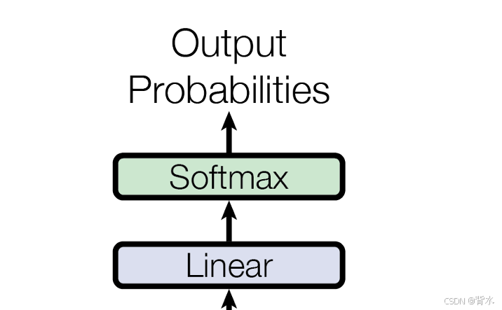
2.2输出部分
线性层softmax层
2.3注意力机制(自注意力机制以及多头注意力机制)
2.3.1 掩码张量
讲解之前,回顾一下线性代数中的“上三角”、“下三角”行矩阵。
-
上三角
[ 1 2 3 4 0 6 7 8 0 0 11 12 0 0 0 16 ] \begin{bmatrix} 1 & 2 & 3 & 4 \\ 0 & 6 & 7 & 8 \\ 0 & 0 & 11 & 12 \\ 0 & 0 & 0 & 16 \end{bmatrix} 1000260037110481216 -
下三角
[ 1 0 0 0 5 6 0 0 9 10 11 0 13 14 15 16 ] \begin{bmatrix} 1 & 0 & 0 & 0 \\ 5 & 6 & 0 & 0 \\ 9 & 10 & 11 & 0 \\ 13 & 14 & 15 & 16 \end{bmatrix} 1591306101400111500016
2.3.1.1 下三角矩阵的作用
- 自回归任务的需求
- 下三角矩阵确保解码器的自注意力机制是因果的(causal),即每个位置的输出只依赖于它
之前的位置,而不依赖于未来的位置。
- 下三角矩阵确保解码器的自注意力机制是因果的(causal),即每个位置的输出只依赖于它
- 屏蔽未来信息
- 在自回归任务(如语言建模、机器翻译)中,模型在生成第 t 个词时,只能依赖于前 t−1个词,而不能依赖于未来的词。
- 下三角矩阵通过将未来位置的信息屏蔽(设置为负无穷或 0),确保模型在计算注意力时只能关注到当前位置及之前的位置。
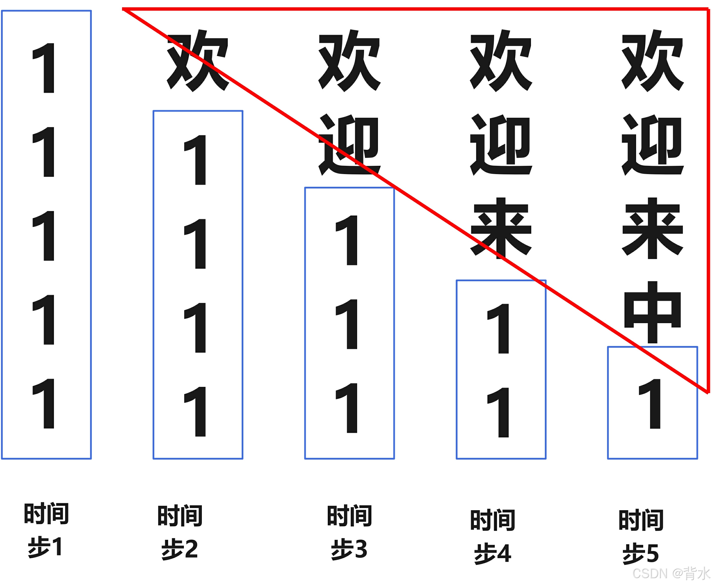
具体例子:
- 生成字符时,
一个时间步一个时间步的解码 - 使用
掩码mask(比如:0表示能看的见, 1表示被这遮掩)希望模型不要使用当前字符和后面的字符。也就是防止模型看到未来信息,用1给他遮掩住)
- 第1个时间步:
5个1表示要生成的5个字符全都被遮掩 - 第2个时间步:只能是看到
“欢”也就是第1个时间步的预测结果 - 第3个时间步:只能是看到
“欢,迎”,也就是第1、2个时间步的预测结果 - 第4个时间步:只能是看到
“欢,迎,来”,也就是第1、2、3个时间步的预测结果 - 第5个时间步:只能是看到
“欢,迎,来,中”,也就是第1、2、3、4个时间步的预测结果
2.3.2 自注意力机制
通俗的讲,自注意力机制中Q==K==V。
2.3.2.1 输入表示
假设输入序列长度为 n n n,每个位置的输入向量维度为 d d d,则输入可以表示为矩阵 X ∈ R n × d X\in \mathbb{R}^{n \times d} X∈Rn×d。
2.3.2.2. 计算查询(Query)、键(Key)和值(Value)
通过线性变换,将输入 X X X 映射为查询矩阵 Q Q Q、键矩阵 K K K 和值矩阵 V V V:
Q = X W Q , K = X W K , V = X W V Q = XW_Q, \quad K = XW_K, \quad V = XW_V Q=XWQ,K=XWK,V=XWV
其中:
- W Q ∈ R d × d k W_Q \in \mathbb{R}^{d \times d_k} WQ∈Rd×dk:查询的权重矩阵。
- W K ∈ R d × d k W_K \in \mathbb{R}^{d \times d_k} WK∈Rd×dk:键的权重矩阵。
- W V ∈ R d × d v W_V \in \mathbb{R}^{d \times d_v} WV∈Rd×dv:值的权重矩阵。
- d k d_k dk 和 d v d_v dv 分别是查询/键和值的维度。
2.3.2.3 计算注意力得分
通过点积计算查询和键之间的相似度,得到注意力得分矩阵 A A A:
A = Q K T d k A = \frac{QK^T}{\sqrt{d_k}} A=dkQKT
其中:
- Q K T QK^T QKT 是一个 n × n n \times n n×n 的矩阵,表示每个位置对所有位置的注意力得分。
- d k \sqrt{d_k} dk 是缩放因子,用于防止点积结果过大,导致梯度消失或爆炸。
2.3.2.4 计算注意力权重
对注意力得分矩阵 A A A 进行 softmax 操作,得到归一化的注意力权重矩阵 α \alpha α:
α = Softmax ( A ) \alpha = \text{Softmax}(A) α=Softmax(A)
其中:
- Softmax 函数对每一行进行归一化,使得每个位置的注意力权重之和为 1。
- 注意力权重 α i j \alpha_{ij} αij 表示第 i i i 个位置对第 j j j 个位置的关注程度。
2.3.2.5 加权求和
使用注意力权重对值矩阵 V V V 进行加权求和,得到每个位置的输出:
Output = α V \text{Output} = \alpha V Output=αV
其中:
- α \alpha α 是 n × n n \times n n×n 的注意力权重矩阵。
- V V V 是 n × d v n \times d_v n×dv 的值矩阵。
- 输出是一个 n × d v n \times d_v n×dv 的矩阵,表示每个位置的新的表示。
2.3.2.6 公式的直观解释
- 查询(Query):表示当前位置的信息。
- 键(Key):表示其他位置的信息。
- 值(Value):表示其他位置的实际内容。
- 注意力得分:通过点积计算查询和键之间的相似度,表示当前位置对其他位置的关注程度。
- 注意力权重:通过 softmax 归一化,使得每个位置的注意力权重之和为 1。
- 加权求和:根据注意力权重对值进行加权求和,得到每个位置的新的表示。
2.3.2.7 具体例子
假设输入序列长度为 3,模型维度 d = 4 d = 4 d=4,则自注意力机制的计算如下:
输入矩阵 X X X:
X = [ 1 2 3 4 5 6 7 8 9 10 11 12 ] X = \begin{bmatrix} 1 & 2 & 3 & 4 \\ 5 & 6 & 7 & 8 \\ 9 & 10 & 11 & 12 \end{bmatrix} X= 159261037114812
假设权重矩阵 W Q , W K , W V W_Q, W_K, W_V WQ,WK,WV 为:
W Q = [ 1 0 0 1 1 0 0 1 ] , W K = [ 0 1 1 0 0 1 1 0 ] , W V = [ 1 0 0 1 1 0 0 1 ] W_Q = \begin{bmatrix} 1 & 0 \\ 0 & 1 \\ 1 & 0 \\ 0 & 1 \end{bmatrix}, \quad W_K = \begin{bmatrix} 0 & 1 \\ 1 & 0 \\ 0 & 1 \\ 1 & 0 \end{bmatrix}, \quad W_V = \begin{bmatrix} 1 & 0 \\ 0 & 1 \\ 1 & 0 \\ 0 & 1 \end{bmatrix} WQ= 10100101 ,WK= 01011010 ,WV= 10100101
则:
Q = X W Q = [ 1 2 5 6 9 10 ] , K = X W K = [ 2 1 6 5 10 9 ] , V = X W V = [ 1 2 5 6 9 10 ] Q = XW_Q = \begin{bmatrix} 1 & 2 \\ 5 & 6 \\ 9 & 10 \end{bmatrix}, \quad K = XW_K = \begin{bmatrix} 2 & 1 \\ 6 & 5 \\ 10 & 9 \end{bmatrix}, \quad V = XW_V = \begin{bmatrix} 1 & 2 \\ 5 & 6 \\ 9 & 10 \end{bmatrix} Q=XWQ= 1592610 ,K=XWK= 2610159 ,V=XWV= 1592610
计算注意力得分
A
=
Q
K
T
d
k
=
1
2
[
1
2
5
6
9
10
]
[
2
6
10
1
5
9
]
=
1
2
[
4
16
28
16
60
104
28
104
180
]
A = \frac{QK^T}{\sqrt{d_k}} = \frac{1}{\sqrt{2}} \begin{bmatrix} 1 & 2 \\ 5 & 6 \\ 9 & 10 \end{bmatrix} \begin{bmatrix} 2 & 6 & 10 \\ 1 & 5 & 9 \end{bmatrix} = \frac{1}{\sqrt{2}} \begin{bmatrix} 4 & 16 & 28 \\ 16 & 60 & 104 \\ 28 & 104 & 180 \end{bmatrix}
A=dkQKT=21
1592610
[2165109]=21
41628166010428104180
计算注意力权重
对
A
A
A 进行 softmax 操作:
α = softmax ( A ) \alpha = \text{softmax}(A) α=softmax(A)
加权求和
使用
α
\alpha
α 对
V
V
V 进行加权求和,得到输出。
2.3.2.7 编码实现
def attention(query, key, value, mask=None, dropout=None):
    # 1 求查询张量特征尺寸大小 d_k
    d_k = query.size()[-1]

    # 2 求查询张量q的权重分布scores  q@k^T /math.sqrt(d_k) /key.transpose(-1, -2)
    # 形状[2,4,512] @ [2,512,4] --->[2,4,4]
    scores = torch.matmul(query, key.transpose(-1, -2)) / math.sqrt(d_k)

    # 3 是否对权重分布scores进行mask scores.masked_fill(c == 0, -1e9)
    if mask is not None:
        scores = scores.masked_fill(mask==0, -1e9)  # 根据mask矩阵 对scores句子进行掩码

    # 4 求查询张量q的权重分布 p_attn F.softmax()
    p_attn = F.softmax(scores, dim=-1)

    # 5 是否对p_attn进行dropout if dropout is not None:
    if dropout is not None:
        p_attn = dropout(p_attn)

    # 6 求查询张量q的注意力结果表示 [2,4,4]@[2,4,512] --->[2,4,512]
    # 7 返回q的注意力结果表示 q的权重分布
    return  torch.matmul(p_attn, value), p_attn


def dm01_test_attention():

    d_model = 512  # 词嵌入维度是512维
    vocab = 1000  # 词表大小是1000

    # 输入x 是一个使用Variable封装的长整型张量, 形状是2 x 4
    x = Variable(torch.LongTensor([[100, 2, 421, 508],
                                   [491, 998, 1, 221]]))
    my_embeddings = Embeddings(d_model, vocab)
    x = my_embeddings(x)

    dropout = 0.1  # 置0比率为0.1
    max_len = 60  # 句子最大长度

    my_pe = PositionalEncoding(d_model, dropout, max_len)
    pe_result = my_pe(x)

    query = key = value = pe_result  # torch.Size([2, 4, 512])

    print('没有使用mask矩阵对 注意力分布进行处理')
    attn1, p_attn1 = attention(query, key, value, mask=None, dropout=None)
    print('注意力结果表示attn1--->', attn1.shape, attn1)
    print('注意力权重分布p_attn1--->', p_attn1.shape, '\n', p_attn1)

    print('使用mask对注意力分布进行处理,注意:这里的mask矩阵是一个全零的矩阵')
    # mask 2*4*4
    mask_zero = torch.zeros(2, 4, 4)
    attn2, p_attn2 = attention(query, key, value, mask=mask_zero, dropout=None)
    print('注意力结果表示attn2--->', attn2.shape, attn2)
    print('注意力权重分布p_attn2--->', p_attn2.shape, '\n', p_attn2)
2.3.2.8 意义解释
假如现在有一个句子[[欢迎,来,到,北京],[欢迎,来,到,上海]]。如果一个单词用8个维度表示,那么可以有下面的张量:
[[[-1.9052, -0.9970,  2.4629, -0.9832,  0.5912,  0.7575, -1.8449, -2.2885],
         [-1.0458,  0.8641,  0.9074,  0.2570,  2.1946,  0.6371, -0.3272,-0.3470],
         [ 0.1827, -0.1038,  1.4048, -0.1738,  0.4960, -0.2144, -1.6113,-1.3831],
         [-0.8744, -0.9542, -1.7613,  0.6556,  0.6225,  0.8198, -0.3386, -1.3912]],

        [[-1.9859,  1.5068,  1.8134,  0.2302,  0.8836,  2.6075,  0.0109, -0.4834],
         [ 0.0526, -0.8190, -1.6013,  0.6656, -0.9374, -1.0759,  0.1085,0.6963],
         [-1.1066,  1.4148,  0.0370,  0.0127, -1.2052, -0.9551, -0.4569,1.8279],
         [ 1.3182,  0.0177,  2.0565,  0.1859, -0.7157, -1.5397,  1.3168,0.4910]]]
因为上面有一个公式为
Q
K
T
QK^T
QKT,下面来解释其具体的含义:
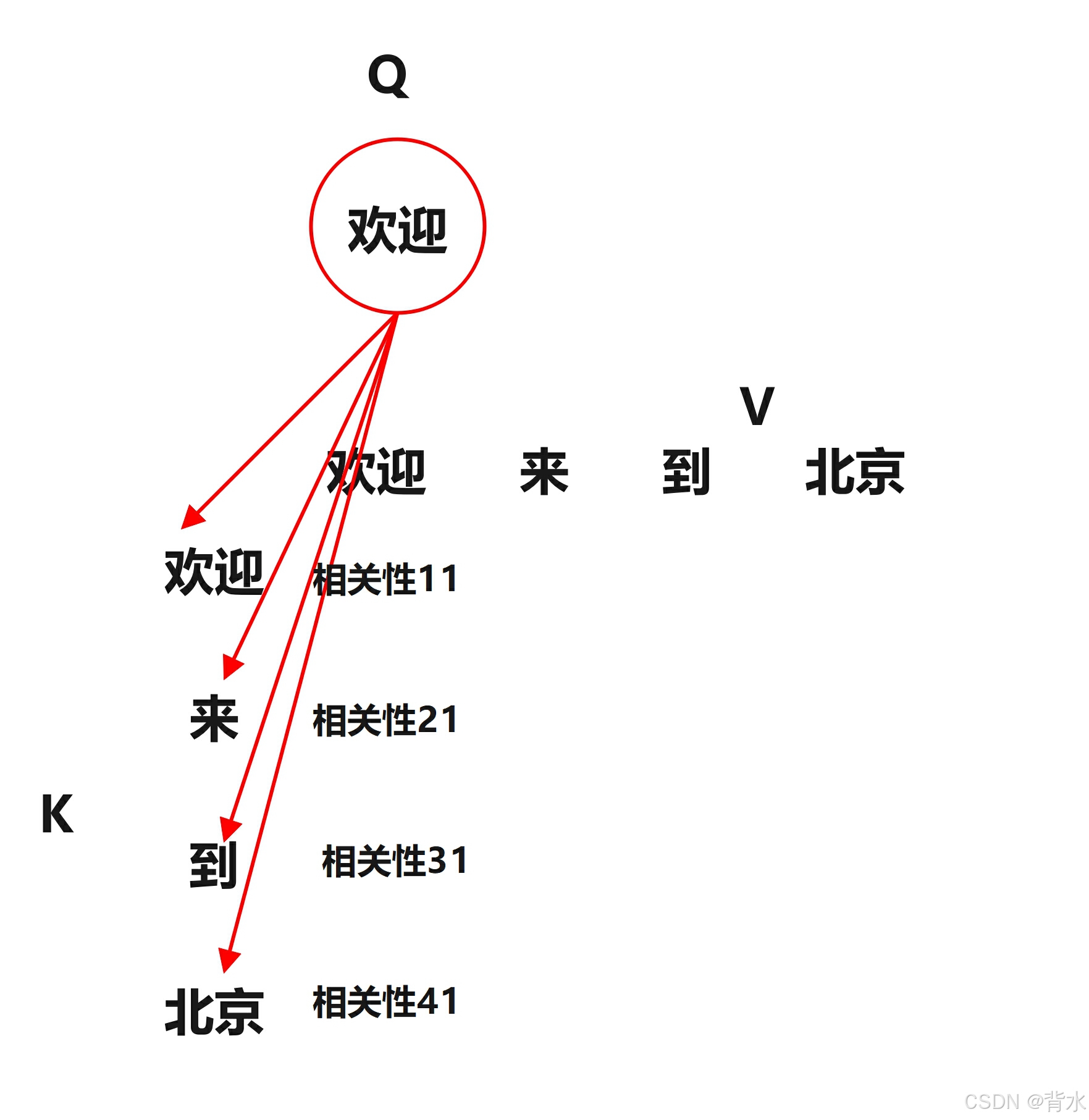
如果这个时间步拿到的是欢迎,想要将其送入模型,还需要计算其在这个句子中“关注哪些词”,比如下面,此时“欢迎”的词向量就是Q,需要拿这个Q与其所处的句子中的词(K)计算相关性(提取特征)。如下面:
Q--欢迎;Q--来;Q--到;Q--北京。当下一次需要拿“来”的时候同样将其与句子中的词做一下相关性计算。
上面公式完成前后,数据的形状变化如下:
- 假设
Q.shape = [batch,seq_len,dimWord] - 其中
batch为批次大小 seqlen为一个句子的长度dimWord为一个单词表示的维度
因为 Q = K = V Q=K=V Q=K=V, Q . s h a p e = [ b a t c h , s e q l e n , d i m W o r d ] Q.shape=[batch,seqlen,dimWord] Q.shape=[batch,seqlen,dimWord]
所以 K T . s h a p e = [ b a t c h , d i m W o r d , s e q l e n ] K^T.shape=[batch,dimWord,seqlen] KT.shape=[batch,dimWord,seqlen]
那么 [ b a t c h , s e q l e n , d i m W o r d ] × [ b a t c h , d i m W o r d , s e q l e n ] = [ b a t c h , s e q l e n , s e q l e n ] [batch,seqlen,dimWord] \times[batch,dimWord,seqlen]=[batch,seqlen,seqlen] [batch,seqlen,dimWord]×[batch,dimWord,seqlen]=[batch,seqlen,seqlen]
接下来是一个Softmax层计算分数(以具体数字为例)
Softmax 会将 Q K T QK^T QKT 的每一行(即每个词与其他词的相关性分数)转换为概率分布。
- 输入:
Q
K
T
QK^T
QKT的形状为
[batch, seq_len, seq_len] - 经过 Softmax 后:形状仍然是
[batch, seq_len, seq_len],但每一行的值被转换为概率分布。 -
V
V
V的形状为
[batch, seq_len, dimWord] - 最终输出:形状为
[batch, seq_len, dimWord]
Softmax 的公式为:
Softmax
(
x
i
)
=
e
x
i
∑
j
=
1
n
e
x
j
\text{Softmax}(x_i) = \frac{e^{x_i}}{\sum_{j=1}^{n} e^{x_j}}
Softmax(xi)=∑j=1nexjexi
以第一个句子为例,假设
Q
K
T
QK^T
QKT 的第一个句子为(去掉batch这个维度):
Q
K
T
=
[
21.2206
6.2903
1.2201
0.8742
6.2903
7.1234
1.5678
1.2345
1.2201
1.5678
5.6789
0.9876
0.8742
1.2345
0.9876
4.5678
]
QK^T = \begin{bmatrix} 21.2206 & 6.2903 & 1.2201 & 0.8742 \\ 6.2903 & 7.1234 & 1.5678 & 1.2345 \\ 1.2201 & 1.5678 & 5.6789 & 0.9876 \\ 0.8742 & 1.2345 & 0.9876 & 4.5678 \end{bmatrix}
QKT=
21.22066.29031.22010.87426.29037.12341.56781.23451.22011.56785.67890.98760.87421.23450.98764.5678
对每一行进行 Softmax 操作。以第一行为例:
Softmax
(
[
21.2206
,
6.2903
,
1.2201
,
0.8742
]
)
\text{Softmax}([21.2206, 6.2903, 1.2201, 0.8742])
Softmax([21.2206,6.2903,1.2201,0.8742])
计算过程:
- 计算指数:
e 21.2206 = 1.63 × 1 0 9 e 6.2903 = 540.49 e 1.2201 = 3.39 e 0.8742 = 2.40 e^{21.2206} = 1.63 \times 10^9 \\ e^{6.2903} = 540.49 \\ e^{1.2201} = 3.39 \\ e^{0.8742} = 2.40 e21.2206=1.63×10⁹e6.2903=540.49e1.2201=3.39e0.8742=2.40 - 计算分母(总和):
sum = 1.63 × 1 0 9 + 540.49 + 3.39 + 2.40 = 1.63 × 1 0 9 \text{sum} = 1.63 \times 10^9 + 540.49 + 3.39 + 2.40 = 1.63 \times 10^9 sum=1.63×10⁹+540.49+3.39+2.40=1.63×10⁹ - 计算 Softmax 分数:
Softmax ( 21.2206 ) = 1.63 × 1 0 9 1.63 × 1 0 9 = 1.0 Softmax ( 6.2903 ) = 540.49 1.63 × 1 0 9 ≈ 0.0 Softmax ( 1.2201 ) = 3.39 1.63 × 1 0 9 ≈ 0.0 Softmax ( 0.8742 ) = 2.40 1.63 × 1 0 9 ≈ 0.0 \text{Softmax}(21.2206) = \frac{1.63 \times 10^9}{1.63 \times 10^9} = 1.0 \\ \text{Softmax}(6.2903) = \frac{540.49}{1.63 \times 10^9} \approx 0.0 \\ \text{Softmax}(1.2201) = \frac{3.39}{1.63 \times 10^9} \approx 0.0 \\ \text{Softmax}(0.8742) = \frac{2.40}{1.63 \times 10^9} \approx 0.0 Softmax(21.2206)=1.63×1091.63×109=1.0Softmax(6.2903)=1.63×109540.49≈0.0Softmax(1.2201)=1.63×1093.39≈0.0Softmax(0.8742)=1.63×1092.40≈0.0
因此,第一行的 Softmax 结果为:
[
1.0
,
0.0
,
0.0
,
0.0
]
[1.0, 0.0, 0.0, 0.0]
[1.0,0.0,0.0,0.0]
同理,对其他行进行 Softmax 操作,最终得到 [batch, seq_len, seq_len]形状的数据:
Softmax
(
Q
K
T
)
=
[
1.0
0.0
0.0
0.0
0.0
1.0
0.0
0.0
0.0
0.0
1.0
0.0
0.0
0.0
0.0
1.0
]
\text{Softmax}(QK^T) = \begin{bmatrix} 1.0 & 0.0 & 0.0 & 0.0 \\ 0.0 & 1.0 & 0.0 & 0.0 \\ 0.0 & 0.0 & 1.0 & 0.0 \\ 0.0 & 0.0 & 0.0 & 1.0 \end{bmatrix}
Softmax(QKT)=
1.00.00.00.00.01.00.00.00.00.01.00.00.00.00.01.0
分数矩阵与
V
V
V 的矩阵乘法
接下来,将 Softmax 后的分数矩阵与
V
V
V进行矩阵乘法。假设
V
V
V的形状为 [batch, seq_len, dimWord],其值与
Q
Q
Q和
K
K
K相同。
矩阵乘法的规则是:
Attention Output
=
Softmax
(
Q
K
T
)
×
V
\text{Attention Output} = \text{Softmax}(QK^T) \times V
Attention Output=Softmax(QKT)×V
其中:
-
Softmax
(
Q
K
T
)
\text{Softmax}(QK^T)
Softmax(QKT) 的形状为
[batch, seq_len, seq_len] -
V
V
V 的形状为
[batch, seq_len, dimWord] - 输出形状为
[batch, seq_len, dimWord]
以第一个句子为例(去除了batch这个维度):
Softmax
(
Q
K
T
)
=
[
1.0
0.0
0.0
0.0
0.0
1.0
0.0
0.0
0.0
0.0
1.0
0.0
0.0
0.0
0.0
1.0
]
\text{Softmax}(QK^T) = \begin{bmatrix} 1.0 & 0.0 & 0.0 & 0.0 \\ 0.0 & 1.0 & 0.0 & 0.0 \\ 0.0 & 0.0 & 1.0 & 0.0 \\ 0.0 & 0.0 & 0.0 & 1.0 \end{bmatrix}
Softmax(QKT)=
1.00.00.00.00.01.00.00.00.00.01.00.00.00.00.01.0
V = [ [ − 1.9052 , − 0.9970 , 2.4629 , − 0.9832 , 0.5912 , 0.7575 , − 1.8449 , − 2.2885 ] [ − 1.0458 , 0.8641 , 0.9074 , 0.2570 , 2.1946 , 0.6371 , − 0.3272 , − 0.3470 ] [ 0.1827 , − 0.1038 , 1.4048 , − 0.1738 , 0.4960 , − 0.2144 , − 1.6113 , − 1.3831 ] [ − 0.8744 , − 0.9542 , − 1.7613 , 0.6556 , 0.6225 , 0.8198 , − 0.3386 , − 1.3912 ] ] V = \begin{bmatrix} [-1.9052, -0.9970, 2.4629, -0.9832, 0.5912, 0.7575, -1.8449, -2.2885] \\ [-1.0458, 0.8641, 0.9074, 0.2570, 2.1946, 0.6371, -0.3272, -0.3470] \\ [ 0.1827, -0.1038, 1.4048, -0.1738, 0.4960, -0.2144, -1.6113, -1.3831] \\ [-0.8744, -0.9542, -1.7613, 0.6556, 0.6225, 0.8198, -0.3386, -1.3912] \end{bmatrix} V= [−1.9052,−0.9970,2.4629,−0.9832,0.5912,0.7575,−1.8449,−2.2885][−1.0458,0.8641,0.9074,0.2570,2.1946,0.6371,−0.3272,−0.3470][0.1827,−0.1038,1.4048,−0.1738,0.4960,−0.2144,−1.6113,−1.3831][−0.8744,−0.9542,−1.7613,0.6556,0.6225,0.8198,−0.3386,−1.3912]
因为
Softmax
(
Q
K
T
)
\text{Softmax}(QK^T)
Softmax(QKT) 是单位矩阵,所以结果与
V
V
V相同。
这里为什么
Softmax
(
Q
K
T
)
\text{Softmax}(QK^T)
Softmax(QKT) 是单位矩阵,这是因为自己和自己的相关性最大!!!!需要后面反向传播调整参数。
2.3.3 多头自注意力机制
多头自注意力机制是在自注意力机制上面的改进。
概念
- 多头注意力机制:
- 多头注意力机制将自注意力机制扩展到多个“头”,每个头独立学习不同的注意力模式。
- 具体步骤包括:
- 线性变换:将输入序列通过不同的线性变换生成多组查询、键和值。
- 计算注意力:每个头独立计算注意力权重并加权求和。
- 拼接和线性变换:将所有头的输出拼接,并通过线性变换得到最终输出。
作用
-
捕捉多种依赖关系:
- 多头注意力机制允许模型同时关注输入序列的不同部分,捕捉多种依赖关系,提升表达能力。
-
增强模型泛化能力:
- 通过并行计算多个注意力头,模型能够学习到更丰富的特征表示,增强泛化能力。
-
提高计算效率:
- 多头注意力机制可以并行计算,充分利用硬件资源,提高计算效率。
-
支持长距离依赖:
- 自注意力机制能够直接捕捉序列中任意两个元素的关系,多头注意力机制进一步增强了这一能力,尤其在处理长序列时表现优异。
2.3.3.1 多头自注意力机制原理图展示
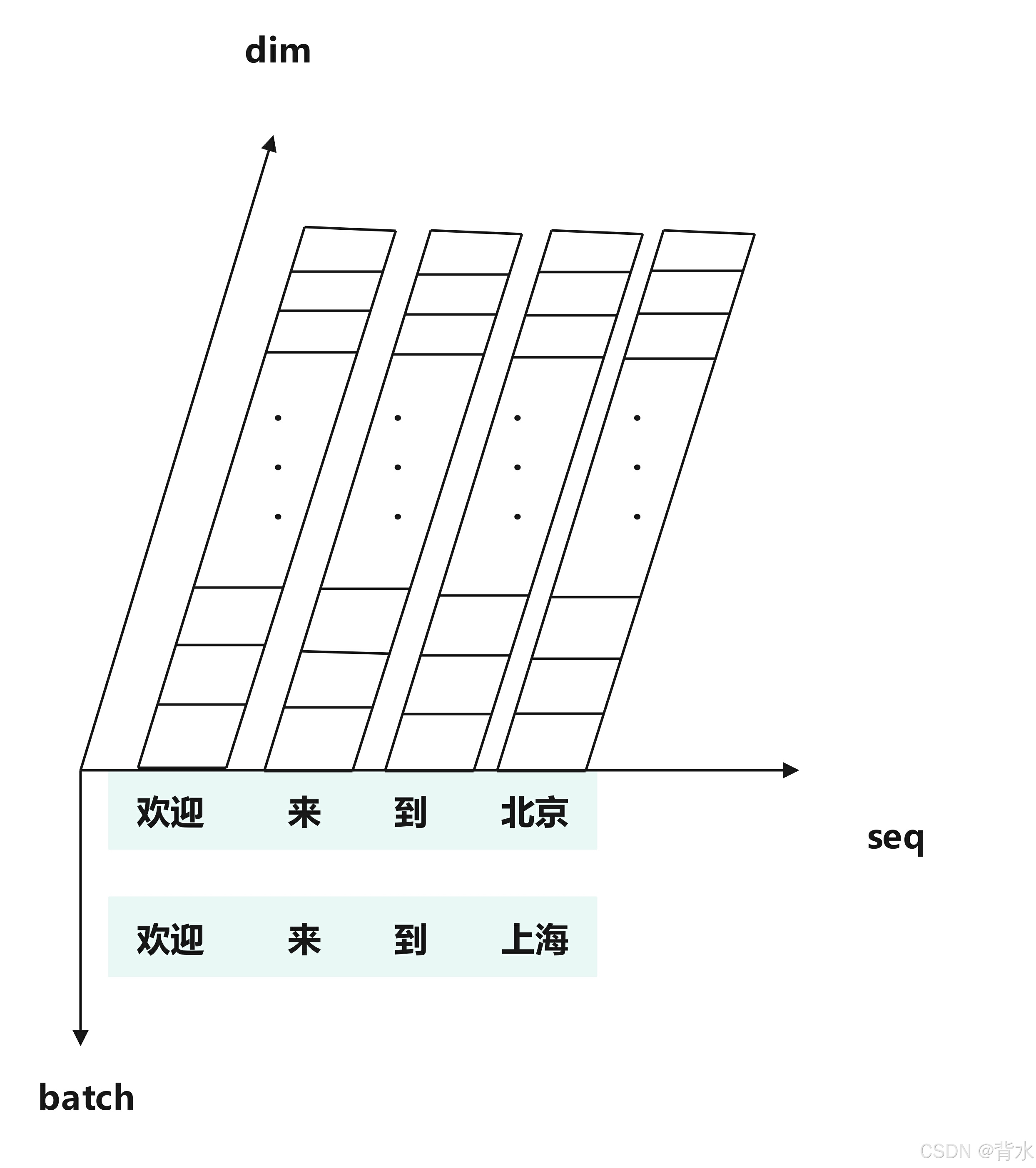
自注意力机制是将整个Q放入attention中,如下图(batch维度是句子个数,seq维度是每个句子的单词个数,dim维度是每个单词的维度):
多注意力机制的策略是按照dim维度,将数据划分为多个‘数据块’,分别进行QKV运算,然后整合在一起。`
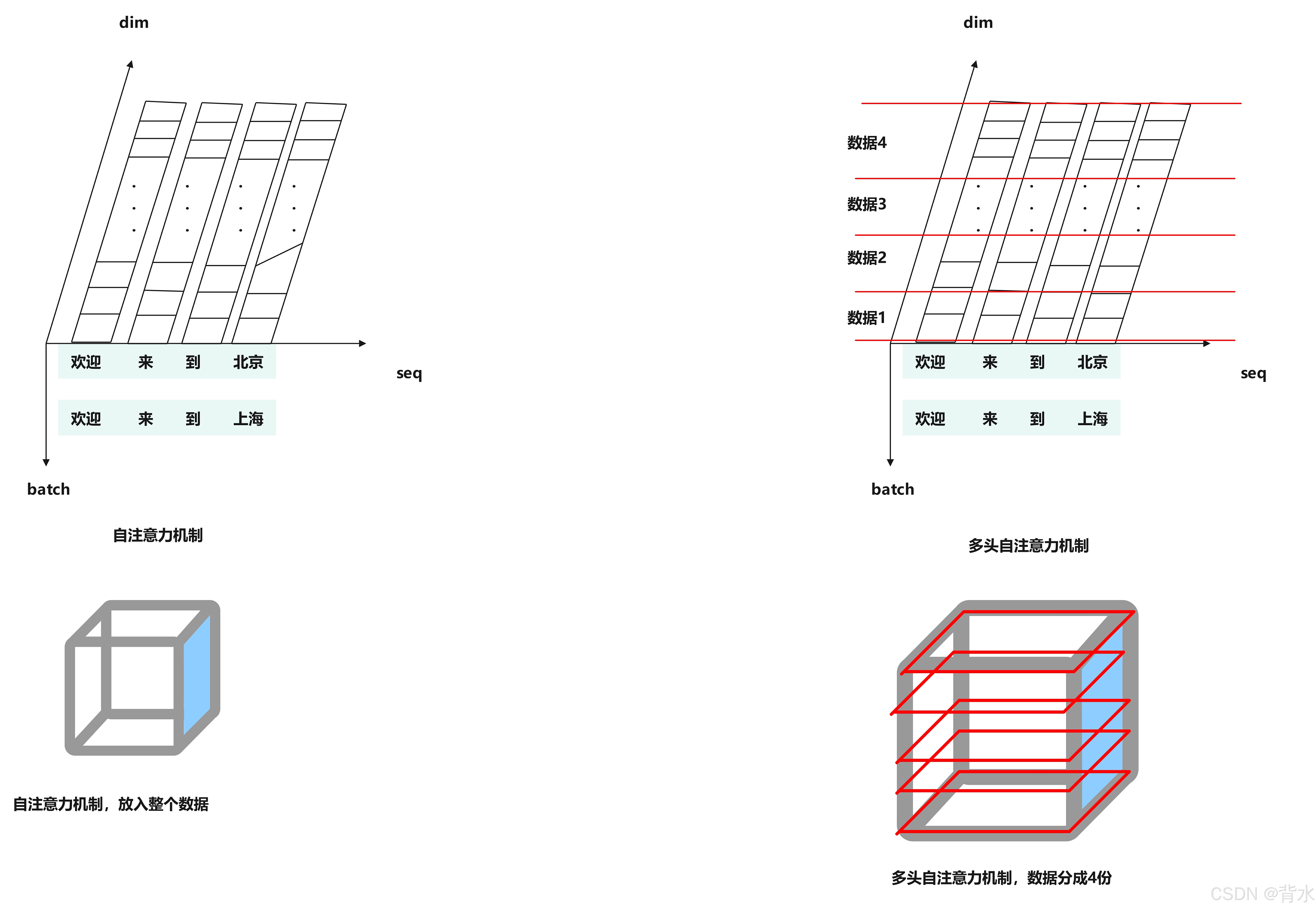
如下图,将Q、K、V分别按照dim维度划分,然后按照对应的数据分别进行QKV运算。
2.3.3.2 多头自注意力机制数据流展示
多头自注意力机制实现流程分为下面几个步骤:
- 线性变换:QKV分别输入到
线性层 - view切分:特征做多头切分, 比如:
512个特征切分成4个头,每个头128个特征 - attention操作:通过attention函数进行多头特征提取
- Concat操作:合并多头特征提取结果
- 线性层变换,最后的得到我们想要的数据形状
假如现在有:[欢迎,来,到,北京]、[欢迎,来,到,上海]这两个句子,每个句子由4个单词组成,每个单词由512个特征组成。那么原数据的形状就是(2,4,512)。为了方便区分数据形状,这里不是和上面一样切分为4个头,而是切分为8个头。
这里需要解释一下,为什么需要使用transpose交换维度。先从切分多头后的数据形状说起,(2,4,8,64),这里的8只是8个数据块(dim维度方面的数据块)。注意力机制的目的是提取单词在句子中的特征,如果将8放在后面,那么提取特征时,这个4(一个句子的长度,单词数量)就会被疏远,若将4和64放的“更近”一些,进行注意力提取的时候,容易提取单词在句子中的含义,因此在进行注意力机制计算时,需要将这个句子中单词数量4向更高的维度放。
2.3.3.2 多头自注意力机制代码实现
def attention(query, key, value, mask=None, dropout=None):
    # 1 求查询张量特征尺寸大小 d_k
    d_k = query.size()[-1]

    # 2 求查询张量q的权重分布scores  q@k^T /math.sqrt(d_k) /key.transpose(-1, -2)
    # 形状[2,4,512] @ [2,512,4] --->[2,4,4]
    scores = torch.matmul(query, key.transpose(-1, -2)) / math.sqrt(d_k)

    # 3 是否对权重分布scores进行mask scores.masked_fill(c == 0, -1e9)
    if mask is not None:
        scores = scores.masked_fill(mask == 0, -1e9)  # 根据mask矩阵 对scores句子进行掩码

    # 4 求查询张量q的权重分布 p_attn F.softmax()
    p_attn = F.softmax(scores, dim=-1)

    # 5 是否对p_attn进行dropout if dropout is not None:
    if dropout is not None:
        p_attn = dropout(p_attn)

    # 6 求查询张量q的注意力结果表示 [2,4,4]@[2,4,512] --->[2,4,512]
    # 7 返回q的注意力结果表示 q的权重分布
    return torch.matmul(p_attn, value), p_attn


def clones(module, N):
    """
    因为多头自注意力机制一共需要4个线性层,所以这里创建一个线性层组
    :param module: 需要复制的模型
    :param N: 需要复制模型的格式
    :return:  模型列表
    """
    return nn.ModuleList([copy.deepcopy(module) for _ in range(N)])


class MultiHeadedAttention(nn.Module):
    def __init__(self, head_num, embedding_dim, dropout=0.1):
        super(MultiHeadedAttention, self).__init__()
        # 每个头特征尺寸大小self.head_size
        self.head_size = embedding_dim // head_num
        # 多少个头
        self.head_num = head_num
        # 线性层列表
        self.linearList = clones(nn.Linear(embedding_dim, embedding_dim), 4)  # 输入多少个特征,输出多少个特征(形状不变)
        # 注意力权重分布self.attn=None  dropout层self.dropout=nn.Dropout(p=dropout)
        self.attn = None
        self.dropout = nn.Dropout(p=dropout)  # 随机失活层,方便微调

        # 分开写
        # self.linear1 = nn.Linear(embedding_dim, embedding_dim)
        # self.linear2 = nn.Linear(embedding_dim, embedding_dim)
        # self.linear3 = nn.Linear(embedding_dim, embedding_dim)
        # self.linear4 = nn.Linear(embedding_dim, embedding_dim)

    def forward(self, query, key, value, mask=None, dropout=0.1):
        # 掩码增加一个维度[8,4,4] -->[1,8,4,4] 求多少批次batch_size
        if mask is not None:
            mask = mask.unsqueeze(0)
        batch_size = query.size()[0]  # 求多少批次batch_size

        # 数据经过线性层 切成8个头,view(batch_size, -1, self.head, self.d_k), transpose(1,2)数据形状变化
        #     数据形状变化[2,4,512] ---> [2,4,8,64] ---> [2,8,4,64]
        query, key, value = [model(x).view(batch_size, -1, self.head_num, self.head_size).transpose(1, 2)
                             for model, x in zip(self.linearList, (query, key, value))]
        # 分开写
        # query = self.linear1(query)
        # key = self.linear2(key)
        # value = self.linear3(value)
        #
        # query = query.reshape(batch_size, -1, self.head_num, self.head_size)
        # key = key.reshape(batch_size, -1, self.head_num, self.head_size)
        # value = value.reshape(batch_size, -1, self.head_num, self.head_size)

        # 各个头 一起送入到attention函数中求 query_plus, self.attn
        # attention([2,8,4,64],[2,8,4,64],[2,8,4,64],[1,8,4,4]) ==> x[2,8,4,64], self.attn[2,8,4,4]]
        query_plus, self.attn = attention(query, key, value, mask=mask)

        # 2-4 数据形状再变化回来 x.transpose(1,2).contiguous().view(batch_size, -1, self.head*self.d_k)
        # 数据形状变化 [2,8,4,64] ---> [2,4,8,64] ---> [2,4,512]
        query_plus = query_plus.transpose(1, 2).contiguous().view(batch_size, -1, self.head_size * self.head_num)

        #  返回最后线性层结果 return self.linears[-1](query_plus)
        query_plus = self.linearList[-1](query_plus)
        return query_plus


def test_MultiHeadedAttention():
    d_model = 512  # 词嵌入维度是512维
    vocab = 1000  # 词表大小是1000

    # 这个数据是经过词嵌入+位置编码器层以后的数据 (加了位置信息以后的数据)
    pe_result = torch.randn(2, 4, 512)

    query = key = value = pe_result  # torch.Size([2, 4, 512])

    # 实例化 MultiHeadedAttention对象
    mha_obj = MultiHeadedAttention(head_num=8, embedding_dim=512, dropout=0.1)
    x = mha_obj(query, key, value)
    print('多头注意机制后的x', x.shape)
    print('多头注意力机制的注意力权重分布', mha_obj.attn.shape)


if __name__ == '__main__':
    test_MultiHeadedAttention()
运行结果:
多头注意机制后的x torch.Size([2, 4, 512])
多头注意力机制的注意力权重分布 torch.Size([2, 8, 4, 4])
下面举出一个为什么4维张量仍然可以放入attention中:
假设:
-
batch_size = 2(2 个样本) -
num_heads = 2(2 个头) -
seq_len = 3(序列长度为 3) -
head_dim = 2(每个头的维度为 2) -
query:形状为[2, 2, 3, 2] -
key:形状为[2, 2, 3, 2] -
value:形状为[2, 2, 3, 2]
具体数据如下:
import torch

# 定义 query, key, value
query = torch.tensor([
    [
        [[1, 2], [3, 4], [5, 6]],  # 第 1 个样本,第 1 个头
        [[7, 8], [9, 10], [11, 12]]  # 第 1 个样本,第 2 个头
    ],
    [
        [[13, 14], [15, 16], [17, 18]],  # 第 2 个样本,第 1 个头
        [[19, 20], [21, 22], [23, 24]]  # 第 2 个样本,第 2 个头
    ]
])

key = torch.tensor([
    [
        [[1, 2], [3, 4], [5, 6]],  # 第 1 个样本,第 1 个头
        [[7, 8], [9, 10], [11, 12]]  # 第 1 个样本,第 2 个头
    ],
    [
        [[13, 14], [15, 16], [17, 18]],  # 第 2 个样本,第 1 个头
        [[19, 20], [21, 22], [23, 24]]  # 第 2 个样本,第 2 个头
    ]
])

value = torch.tensor([
    [
        [[1, 2], [3, 4], [5, 6]],  # 第 1 个样本,第 1 个头
        [[7, 8], [9, 10], [11, 12]]  # 第 1 个样本,第 2 个头
    ],
    [
        [[13, 14], [15, 16], [17, 18]],  # 第 2 个样本,第 1 个头
        [[19, 20], [21, 22], [23, 24]]  # 第 2 个样本,第 2 个头
    ]
])
注意力分数的计算公式为:
scores = Q K T d k \text{scores} = \frac{Q K^T}{\sqrt{d_k}} scores=dkQKT
其中:
-
Q
Q
Q 是
query,形状为[2, 2, 3, 2]。 -
K
K
K 是
key,形状为[2, 2, 3, 2]。 -
K
T
K^T
KT 是
key的转置,形状为[2, 2, 2, 3]。
使用 key.transpose(-1, -2) 对 key 进行转置,key_transposed 的形状为 [2, 2, 2, 3]。:
key_transposed = key.transpose(-1, -2),
使用 torch.matmul 计算 query 和 key_transposed 的点积,结果的形状为 [2, 2, 3, 3]。:
scores = torch.matmul(query, key_transposed)
具体计算
以第 1 个样本、第 1 个头为例:
query的第 1 个头数据:
Q 1 = [ 1 2 3 4 5 6 ] Q_1 = \begin{bmatrix} 1 & 2 \\ 3 & 4 \\ 5 & 6 \end{bmatrix} Q1= 135246 key_transposed的第 1 个头数据:
K 1 T = [ 1 3 5 2 4 6 ] K_1^T = \begin{bmatrix} 1 & 3 & 5 \\ 2 & 4 & 6 \end{bmatrix} K1T=[123456]- 计算点积:
Q 1 K 1 T = [ 1 ⋅ 1 + 2 ⋅ 2 1 ⋅ 3 + 2 ⋅ 4 1 ⋅ 5 + 2 ⋅ 6 3 ⋅ 1 + 4 ⋅ 2 3 ⋅ 3 + 4 ⋅ 4 3 ⋅ 5 + 4 ⋅ 6 5 ⋅ 1 + 6 ⋅ 2 5 ⋅ 3 + 6 ⋅ 4 5 ⋅ 5 + 6 ⋅ 6 ] = [ 5 11 17 11 25 39 17 39 61 ] Q_1 K_1^T = \begin{bmatrix} 1 \cdot 1 + 2 \cdot 2 & 1 \cdot 3 + 2 \cdot 4 & 1 \cdot 5 + 2 \cdot 6 \\ 3 \cdot 1 + 4 \cdot 2 & 3 \cdot 3 + 4 \cdot 4 & 3 \cdot 5 + 4 \cdot 6 \\ 5 \cdot 1 + 6 \cdot 2 & 5 \cdot 3 + 6 \cdot 4 & 5 \cdot 5 + 6 \cdot 6 \end{bmatrix} = \begin{bmatrix} 5 & 11 & 17 \\ 11 & 25 & 39 \\ 17 & 39 & 61 \end{bmatrix} Q1K1T= 1⋅1+2⋅23⋅1+4⋅25⋅1+6⋅21⋅3+2⋅43⋅3+4⋅45⋅3+6⋅41⋅5+2⋅63⋅5+4⋅65⋅5+6⋅6 = 51117112539173961
缩放
将点积结果除以
d
k
\sqrt{d_k}
dk(这里
d
k
=
2
d_k = 2
dk=2):
scores = scores / torch.sqrt(torch.tensor(2.0))
计算注意力权重
对 scores 应用 Softmax,得到注意力权重:
import torch.nn.functional as F

attn_weights = F.softmax(scores, dim=-1)
attn_weights 的形状为 [2, 2, 3, 3]。
计算加权和
将注意力权重与 value 相乘,得到加权和:
output = torch.matmul(attn_weights, value)
output 的形状为 [2, 2, 3, 2]。
以第 1 个样本、第 1 个头为例:
attn_weights的第 1 个头数据:
A 1 = [ 0.2 0.3 0.5 0.1 0.6 0.3 0.4 0.4 0.2 ] A_1 = \begin{bmatrix} 0.2 & 0.3 & 0.5 \\ 0.1 & 0.6 & 0.3 \\ 0.4 & 0.4 & 0.2 \end{bmatrix} A1= 0.20.10.40.30.60.40.50.30.2 value的第 1 个头数据:
V 1 = [ 1 2 3 4 5 6 ] V_1 = \begin{bmatrix} 1 & 2 \\ 3 & 4 \\ 5 & 6 \end{bmatrix} V1= 135246 - 计算加权和:
A 1 V 1 = [ 0.2 ⋅ 1 + 0.3 ⋅ 3 + 0.5 ⋅ 5 0.2 ⋅ 2 + 0.3 ⋅ 4 + 0.5 ⋅ 6 0.1 ⋅ 1 + 0.6 ⋅ 3 + 0.3 ⋅ 5 0.1 ⋅ 2 + 0.6 ⋅ 4 + 0.3 ⋅ 6 0.4 ⋅ 1 + 0.4 ⋅ 3 + 0.2 ⋅ 5 0.4 ⋅ 2 + 0.4 ⋅ 4 + 0.2 ⋅ 6 ] = [ 3.6 4.8 3.4 4.4 2.6 3.6 ] A_1 V_1 = \begin{bmatrix} 0.2 \cdot 1 + 0.3 \cdot 3 + 0.5 \cdot 5 & 0.2 \cdot 2 + 0.3 \cdot 4 + 0.5 \cdot 6 \\ 0.1 \cdot 1 + 0.6 \cdot 3 + 0.3 \cdot 5 & 0.1 \cdot 2 + 0.6 \cdot 4 + 0.3 \cdot 6 \\ 0.4 \cdot 1 + 0.4 \cdot 3 + 0.2 \cdot 5 & 0.4 \cdot 2 + 0.4 \cdot 4 + 0.2 \cdot 6 \end{bmatrix} = \begin{bmatrix} 3.6 & 4.8 \\ 3.4 & 4.4 \\ 2.6 & 3.6 \end{bmatrix} A1V1= 0.2⋅1+0.3⋅3+0.5⋅50.1⋅1+0.6⋅3+0.3⋅50.4⋅1+0.4⋅3+0.2⋅50.2⋅2+0.3⋅4+0.5⋅60.1⋅2+0.6⋅4+0.3⋅60.4⋅2+0.4⋅4+0.2⋅6 = 3.63.42.64.84.43.6
2.4前馈全连接层
前馈全连接层(Feed-Forward Neural Network, FFN)是神经网络中的一种基本结构,通常用于对输入数据进行非线性变换和特征提取。在 Transformer 模型中,前馈全连接层是每个编码器和解码器模块的重要组成部分,用于对自注意力机制输出的特征进行进一步处理。
2.4.1. 前馈全连接层的结构
前馈全连接层通常由两个线性变换(全连接层)和一个激活函数组成。其结构如下:
- 第一个线性变换:将输入特征从
d_model维度映射到d_ff维度(通常d_ff > d_model)。 - 激活函数:对第一个线性变换的结果应用非线性激活函数(如 ReLU)。
- 第二个线性变换:将激活后的特征从
d_ff维度映射回d_model维度。
用公式表示为:
FFN
(
x
)
=
Linear
2
(
ReLU
(
Linear
1
(
x
)
)
)
\text{FFN}(x) = \text{Linear}_2(\text{ReLU}(\text{Linear}_1(x)))
FFN(x)=Linear2(ReLU(Linear1(x)))
其中:
-
x
x
x是输入,形状为
[batch_size, seq_len, d_model]。 -
Linear
1
\text{Linear}_1
Linear1 是第一个线性变换,权重矩阵形状为
[d_model, d_ff]。 - ReLU \text{ReLU} ReLU是激活函数。
-
Linear
2
\text{Linear}_2
Linear2 是第二个线性变换,权重矩阵形状为
[d_ff, d_model]。
2.4.2. 前馈全连接层的数学公式
假设输入 ( x ) 的形状为 [batch_size, seq_len, d_model],前馈全连接层的计算过程如下:
2.4.2.1 第一个线性变换
将输入
x
x
x 从 d_model 维度映射到 d_ff 维度:
z = x W 1 + b 1 z = x W_1 + b_1 z=xW1+b1
其中:
-
W
1
W_1
W1 是第一个线性变换的权重矩阵,形状为
[d_model, d_ff]。 -
b
1
b_1
b1 是第一个线性变换的偏置向量,形状为
[d_ff]。 -
z
z
z是第一个线性变换的输出,形状为
[batch_size, seq_len, d_ff]。
2.4.2.2 激活函数
对 z z z 应用 ReLU 激活函数:
a = ReLU ( z ) a = \text{ReLU}(z) a=ReLU(z)
其中:
-
a
a
a 是激活后的输出,形状仍为
[batch_size, seq_len, d_ff]。
2.4.2.3 第二个线性变换
将
a
a
a 从 d_ff 维度映射回 d_model 维度:
y = a W 2 + b 2 y = a W_2 + b_2 y=aW2+b2
其中:
-
W
2
W_2
W2 是第二个线性变换的权重矩阵,形状为
[d_ff, d_model]。 -
b
2
b_2
b2 是第二个线性变换的偏置向量,形状为
[d_model]。 -
y
y
y是前馈全连接层的最终输出,形状为
[batch_size, seq_len, d_model]。
2.4.3. 前馈全连接层的作用
前馈全连接层的主要作用是对自注意力机制输出的特征进行进一步的非线性变换和特征提取。具体来说:
- 特征增强:通过非线性激活函数(如 ReLU),前馈全连接层可以增强模型的表达能力,捕捉更复杂的特征。
- 维度变换:通过两个线性变换,前馈全连接层可以将特征从高维空间映射到低维空间,再从低维空间映射回高维空间,从而提取更有意义的特征。
- 独立处理每个位置:前馈全连接层对序列中的每个位置独立处理,因此可以捕捉序列中每个位置的特征。
2.4.4. 代码实现
class PositionwiseFeedForward(nn.Module):
    def __init__(self, d_model, d_ff, dropout=0.1):
        super(PositionwiseFeedForward, self).__init__()

        self.w1 = nn.Linear(d_model, d_ff)
        self.w2 = nn.Linear(d_ff, d_model)
        self.dropout = nn.Dropout(p=dropout)

    def forward(self, x): # w1 [8,512]  -->[8,1024]  ; w2[8,1024]-->[8,512]
        x = self.w1(x)
        x = F.relu(x)
        x = self.dropout(x)
        x = self.w2(x)
        return x
2.5 规范化层
Transformer模型中的规范化层(Normalization Layer)通常采用层归一化(Layer Normalization, LN),用于稳定训练过程并加速收敛。以下是对层归一化的详细解释,包括数学原理和数据形状变化。
2.5.1. 层归一化的作用
层归一化的主要目的是对每一层的输入进行标准化处理,使其均值为0,方差为1。这样可以缓解梯度消失或梯度爆炸问题,提升模型的训练稳定性。
在Transformer中,层归一化通常应用于以下两个地方:
- 多头自注意力层的输出之后。
- 前馈神经网络的输出之后。
2.5.2. 数学原理
层归一化的数学公式如下:
给定输入向量 x = ( x 1 , x 2 , … , x d ) x = (x_1, x_2, \dots, x_d) x=(x1,x2,…,xd),其中 d d d 是特征的维度,层归一化的计算步骤如下:
-
计算均值和方差:
- 均值:
μ = 1 d ∑ i = 1 d x i \mu = \frac{1}{d} \sum_{i=1}^d x_i μ=d1i=1∑dxi - 方差:
σ 2 = 1 d ∑ i = 1 d ( x i − μ ) 2 \sigma^2 = \frac{1}{d} \sum_{i=1}^d (x_i - \mu)^2 σ2=d1i=1∑d(xi−μ)2
- 均值:
-
标准化:
- 对输入进行标准化,使其均值为0,方差为1:
x ^ i = x i − μ σ 2 + ϵ \hat{x}_i = \frac{x_i - \mu}{\sqrt{\sigma^2 + \epsilon}} x^i=σ2+ϵxi−μ
其中, ϵ \epsilon ϵ是一个很小的常数(如 1 0 − 5 10^{-5} 10−5),用于防止除零错误。
- 对输入进行标准化,使其均值为0,方差为1:
-
缩放和平移:
- 引入可学习的参数
γ
\gamma
γ 和
β
\beta
β,对标准化后的结果进行缩放和平移:
y i = γ x ^ i + β y_i = \gamma \hat{x}_i + \beta yi=γx^i+β
其中, γ \gamma γ 和 β \beta β 是可学习的参数,维度与输入 x x x 相同。
- 引入可学习的参数
γ
\gamma
γ 和
β
\beta
β,对标准化后的结果进行缩放和平移:
2.5.3. 数据形状变化
在Transformer中,层归一化的输入和输出形状保持一致。具体来说:
-
输入形状:假设输入是一个形状为
(batch_size, sequence_length, feature_dim)的张量。batch_size:批次大小。sequence_length:序列长度。feature_dim:每个特征的维度。
-
归一化操作:
- 层归一化对每个样本的每个时间步(即
sequence_length维度)独立进行归一化。 - 具体来说,对于每个样本的每个时间步,计算其
feature_dim维度上的均值和方差,然后进行标准化和缩放平移。
- 层归一化对每个样本的每个时间步(即
-
输出形状:输出的形状与输入完全相同,仍然是
(batch_size, sequence_length, feature_dim)。
2.5.4. 代码实现
class LayerNorm(nn.Module):
    def __init__(self, features, eps=1e-6):
        super(LayerNorm, self).__init__()
        self.a2 = nn.Parameter(torch.ones(features))    # 缩放因子
        self.b2 = nn.Parameter(torch.ones(features))    # 偏移因子
        self.eps = eps

    def forward(self, x):
        mean = x.mean(dim=-1, keepdims=True)
        std = x.std(dim=-1, keepdims=True)

        x = self.a2 * (x-mean) / (std + self.eps ) + self.b2
        return  x


def test_LayerNorm():

    # 实例化标准化层
    mylayernorm =  LayerNorm(512)
    print('mylayernorm--->', mylayernorm)

    # 给模型喂数据
    pe_result = torch.randn(2, 4, 512)
    layernorm_result =  mylayernorm(pe_result)
    print('layernorm_result--->', layernorm_result, layernorm_result.shape)
    pass
2.5.5. 广播机制
上面代码(在 x = self.a2 * (x - mean) / (std + self.eps) + self.b2 )自动调用了广播机制,为了方便观察,下面将举出具体的例子:
输入数据
假设输入张量 x 的形状为 (2, 3, 4),即:
- 批次大小
batch_size = 2。 - 序列长度
sequence_length = 3。 - 特征维度
feature_dim = 4。
具体数据如下:
x = [
    # 批次 1
    [
        [1.0, 2.0, 3.0, 4.0],  # 时间步 1
        [2.0, 3.0, 4.0, 5.0],  # 时间步 2
        [3.0, 4.0, 5.0, 6.0]   # 时间步 3
    ],
    # 批次 2
    [
        [4.0, 5.0, 6.0, 7.0],  # 时间步 1
        [5.0, 6.0, 7.0, 8.0],  # 时间步 2
        [6.0, 7.0, 8.0, 9.0]   # 时间步 3
    ]
]
计算均值和标准差
在 LayerNorm 中,均值和标准差是在特征维度(feature_dim)上计算的,并且使用 keepdims=True 保持维度。
(1) 计算均值
对于每个时间步的特征维度,计算均值:
μ
t
=
1
d
∑
j
=
1
d
x
t
j
\mu_t = \frac{1}{d} \sum_{j=1}^d x_{tj}
μt=d1j=1∑dxtj
其中,( d = 4 )(特征维度)。
计算结果:
mean = [
    # 批次 1
    [
        [2.5],  # 时间步 1 的均值
        [3.5],  # 时间步 2 的均值
        [4.5]   # 时间步 3 的均值
    ],
    # 批次 2
    [
        [5.5],  # 时间步 1 的均值
        [6.5],  # 时间步 2 的均值
        [7.5]   # 时间步 3 的均值
    ]
]
形状为 (2, 3, 1)。
(2)计算标准差
对于每个时间步的特征维度,计算标准差:
σ
t
=
1
d
∑
j
=
1
d
(
x
t
j
−
μ
t
)
2
\sigma_t = \sqrt{\frac{1}{d} \sum_{j=1}^d (x_{tj} - \mu_t)^2}
σt=d1j=1∑d(xtj−μt)2
计算结果:
std = [
    # 批次 1
    [
        [1.118],  # 时间步 1 的标准差
        [1.118],  # 时间步 2 的标准差
        [1.118]   # 时间步 3 的标准差
    ],
    # 批次 2
    [
        [1.118],  # 时间步 1 的标准差
        [1.118],  # 时间步 2 的标准差
        [1.118]   # 时间步 3 的标准差
    ]
]
形状为 (2, 3, 1)。
标准化操作
标准化操作的公式为:
x
^
t
j
=
x
t
j
−
μ
t
σ
t
+
ϵ
\hat{x}_{tj} = \frac{x_{tj} - \mu_t}{\sigma_t + \epsilon}
x^tj=σt+ϵxtj−μt
广播机制
x - mean:x的形状为(2, 3, 4),mean的形状为(2, 3, 1)。- 广播机制会将
mean扩展为(2, 3, 4),即每个时间步的均值复制 4 次。
计算结果
标准化后的结果:
x_hat = [
    # 批次 1
    [
        [-1.3416, -0.4472, 0.4472, 1.3416],  # 时间步 1
        [-1.3416, -0.4472, 0.4472, 1.3416],  # 时间步 2
        [-1.3416, -0.4472, 0.4472, 1.3416]   # 时间步 3
    ],
    # 批次 2
    [
        [-1.3416, -0.4472, 0.4472, 1.3416],  # 时间步 1
        [-1.3416, -0.4472, 0.4472, 1.3416],  # 时间步 2
        [-1.3416, -0.4472, 0.4472, 1.3416]   # 时间步 3
    ]
]
形状仍为 (2, 3, 4)。
总结
- 广播机制在
x = self.a2 * (x - mean) / (std + self.eps) + self.b2中的作用:x - mean:将mean的形状(2, 3, 1)广播为(2, 3, 4)。self.a2 * x_hat:将self.a2的形状(4,)广播为(2, 3, 4)。+ self.b2:将self.b2的形状(4,)广播为(2, 3, 4)。
- 最终输出的形状与输入一致,为
(2, 3, 4)。
2.5.5 LayerNorm&BatchNorm
2.5.5.1. Layer Normalization (LayerNorm)
工作原理
LayerNorm 对每个样本的每个时间步的特征维度进行规范化。具体来说:
- 对于一个输入张量
X
X
X(形状为
(batch_size, sequence_length, feature_dim)),LayerNorm 在每个样本的每个时间步上计算特征维度的均值和方差。 - 使用均值和方差对特征进行标准化:
x ^ t j = x t j − μ t σ t 2 + ϵ \hat{x}_{tj} = \frac{x_{tj} - \mu_t}{\sqrt{\sigma_t^2 + \epsilon}} x^tj=σt2+ϵxtj−μt
其中:- μ t \mu_t μt是时间步 t t t 的均值。
- σ t 2 \sigma_t^2 σt2是时间步 t t t 的方差。
- ϵ \epsilon ϵ 是一个很小的常数,用于防止除零错误。
- 对标准化后的结果进行缩放和平移:
y t j = γ j ⋅ x ^ t j + β j y_{tj} = \gamma_j \cdot \hat{x}_{tj} + \beta_j ytj=γj⋅x^tj+βj
其中, γ j \gamma_j γj 和 β j \beta_j βj 是可学习的参数。
适用领域
- 自然语言处理 (NLP):LayerNorm 广泛应用于 Transformer 模型(如 BERT、GPT)中,因为它对序列数据的处理更加稳定。
- 变长序列数据:LayerNorm 不依赖于批次大小,适合处理变长序列数据(如文本、语音)。
- 小批次或单样本训练:LayerNorm 对批次大小不敏感,适合小批次或单样本训练场景。
优点
- 不依赖于批次大小,适合小批次或动态批次训练。
- 对序列数据的处理更加稳定。
- 在 Transformer 等模型中表现优异。
缺点
- 对于卷积神经网络 (CNN),LayerNorm 的效果通常不如 BatchNorm。
2.5.5.2. Batch Normalization (BatchNorm)
工作原理
BatchNorm 对每个特征通道在批次维度上进行规范化。具体来说:
- 对于一个输入张量 ( X )(形状为
(batch_size, channels, height, width)),BatchNorm 在每个特征通道上计算批次维度的均值和方差。 - 使用均值和方差对特征进行标准化:
x ^ i j = x i j − μ j σ j 2 + ϵ \hat{x}_{ij} = \frac{x_{ij} - \mu_j}{\sqrt{\sigma_j^2 + \epsilon}} x^ij=σj2+ϵxij−μj
其中:-
μ
j
\mu_j
μj 是特征通道
j
j
j 的均值。
- σ j 2 \sigma_j^2 σj2 是特征通道 j j j 的方差。 - ϵ \epsilon ϵ 是一个很小的常数,用于防止除零错误。
-
μ
j
\mu_j
μj 是特征通道
j
j
j 的均值。
- 对标准化后的结果进行缩放和平移:
y i j = γ j ⋅ x ^ i j + β j y_{ij} = \gamma_j \cdot \hat{x}_{ij} + \beta_j yij=γj⋅x^ij+βj
其中, γ j \gamma_j γj 和 β j \beta_j βj是可学习的参数。
适用领域
- 计算机视觉 (CV):BatchNorm 广泛应用于卷积神经网络 (CNN) 中,如图像分类、目标检测等任务。
- 大批次训练:BatchNorm 依赖于批次统计量,适合大批次训练场景。
- 固定长度的数据:BatchNorm 对批次大小敏感,适合处理固定长度的数据(如图像)。
优点
- 在卷积神经网络中表现优异,能够加速训练并提高模型性能。
- 对大批次数据的处理更加稳定。
缺点
- 对小批次或动态批次训练不友好,因为批次统计量可能不准确。
- 对序列数据的处理不如 LayerNorm 稳定。
2.5.5.4 LayerNorm 和 BatchNorm 的对比
| 特性 | LayerNorm | BatchNorm |
|---|---|---|
| 规范化维度 | 特征维度(feature_dim) | 批次维度(batch_size) |
| 适用领域 | NLP、序列数据、小批次训练 | CV、固定长度数据、大批次训练 |
| 对批次大小的依赖 | 不依赖 | 依赖 |
| 稳定性 | 对序列数据更稳定 | 对大批次数据更稳定 |
| 计算开销 | 较低 | 较高 |
| 常见模型 | Transformer、BERT、GPT | ResNet、VGG、CNN |
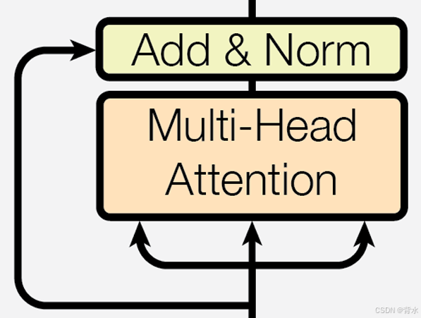
2.6 子层连接结构
上面介绍了多头自注意力机制、前馈全连接、规范化层等。那么现在的问题就是如何将它们连接在一起。这就需要引入子层连接结构。
子层指的是“多头注意力子层或者前馈全连接层”子层连接结构=子层+规范化层+残差连接
如下图,数据先经过子层和规范化层,然后再和数据相加得到新的数据。(有时数据会先经过规范化层,再经过子层)
下面是模型中具体的子层连接结构:
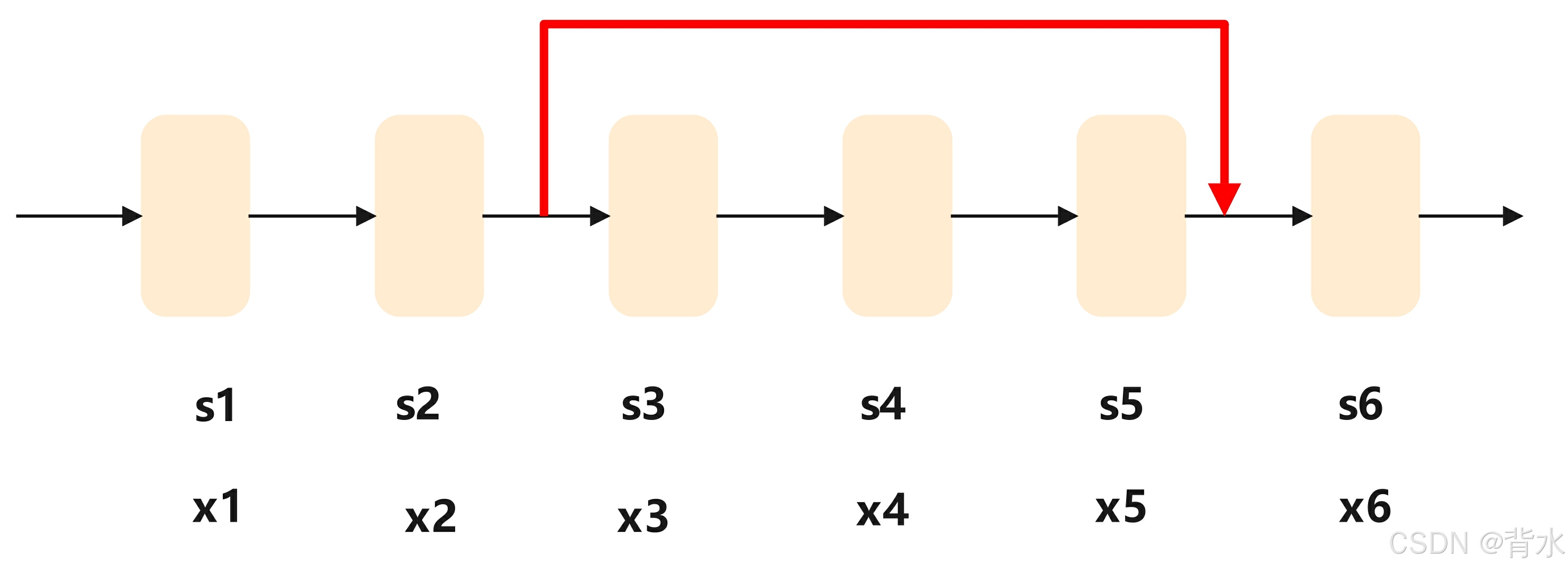
2.6.1. 对于残差连接的解释
上图中有6个层,第
i
i
i个层是
s
i
s_i
si,经过
s
i
s_i
si层后的数据是
x
i
x_i
xi,有这样一种情况,随着层数的增加,在前向传播时,可能会发生
s
3
,
s
4
,
s
5
s_3,s_4,s_5
s3,s4,s5这几个层将
s
2
s_2
s2提取的特征丢弃了,如果不在
s
2
s_2
s2后面加上一个连接到
s
6
s_6
s6前面的线,那么会发生特征丢失的现象。相反,如果加上这条线,即使特征丢失了,那么
s
6
s_6
s6也可以不使用用
s
3
,
s
4
,
s
5
s_3,s_4,s_5
s3,s4,s5提取的特征,而使用
x
2
x_2
x2(因为
x
5
=
f
(
x
4
)
+
x
2
x_5=f(x_4)+x_2
x5=f(x4)+x2)。
2.6.2. 代码实现
class SublayerConnection(nn.Module):
    def __init__(self, features, dropout=0.1):
        super(SublayerConnection, self).__init__()
        self.norm = LayerNorm(features=features)  # 规范化层 ,因为每一个都要用
        self.dropout = nn.Dropout(p=dropout)

    def forward(self, x, sublayer):
        """
        :param x: 输入的数据
        :param sublayer: 可能是注意力机制层函数,也可以能是前馈全连接层函数
        :return: 返回结合后的数据
        """
        x = x + self.dropout(sublayer(self.norm(x)))  # 这里是采用先经过规范化层,再经过子层
        return x


def test_SublayerConnection():
    size = 512
    # 实例化子层连接结构对象
    my_sublayerconnection = SublayerConnection(size)
    print('my_sublayerconnection--->', my_sublayerconnection)

    # 给模型喂数据
    # 准备数据
    x = torch.randn(2, 4, 512)

    # 准备函数的入口地址
    # 实例化多头注意力机制对象
    my_mha = MultiHeadedAttention(8, 512, 0.1)
    # 构建多头注意力机制对象的forward函数的 入口地址
    sublayer = lambda x: my_mha(x, x, x)

    x = my_sublayerconnection(x, sublayer)
    print('x-->', x.shape, x)
运行结果:
my_sublayerconnection---> SublayerConnection(
  (norm): LayerNorm()
  (dropout): Dropout(p=0.1, inplace=False)
)
x--> torch.Size([2, 4, 512]) tensor([[[-0.8942, -0.4785,  0.0998,  ..., -0.2341, -2.1095, -2.0566],
         [ 1.0414, -1.6628,  1.1701,  ..., -1.0048,  0.2592, -1.3312],
         [ 0.2529, -1.6511, -0.3957,  ..., -0.5132,  1.1151,  0.2032],
         [-0.7524,  1.8790, -0.1766,  ..., -0.5492,  0.8182,  0.1722]],

        [[ 0.5965, -0.9109, -0.9878,  ...,  1.1941,  0.5187, -2.2414],
         [-0.1335,  0.2706, -0.4785,  ...,  0.7445,  0.7804, -1.9683],
         [ 0.4043, -0.0054, -0.2924,  ..., -0.0244, -0.0868, -1.8685],
         [-0.3144, -1.9200,  1.0806,  ...,  0.6712,  1.7461, -1.7864]]],
       grad_fn=<AddBackward0>)
2.7编码器部分
- 由
N个编码器层堆叠而成 - 每个编码器层由
两个子层连接结构组成 - 第一个子层连接结构包括一个
多头自注意力子层和规范化层以及一个残差连接 - 第二个子层连接结构包括一个
前馈全连接子层和规范化层以及一个残差连接
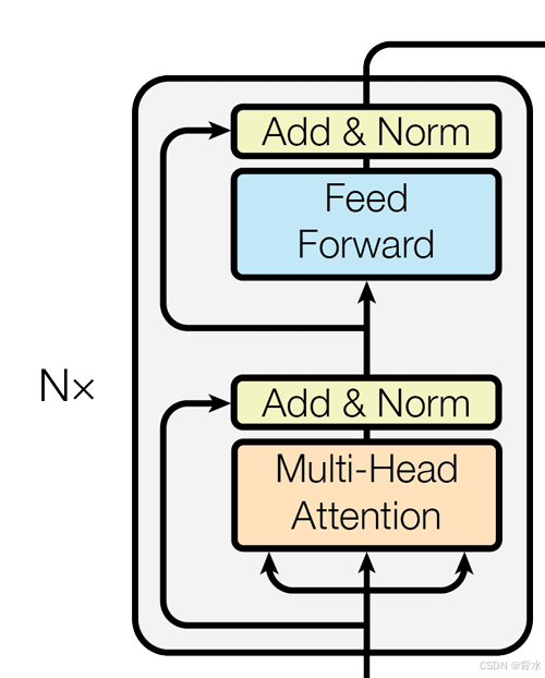
这里假设N = 3
2.7.1. 编码器层实现
一个编码器由 N N N个编码器层组成,下面是一个编码器层的实现代码:
class EncoderLayer(nn.Module):
    def __init__(self, feature, self_attention, feed_forward, dropout):
        super().__init__()
        """
        :param feature: 一个单词的维度
        :param self_attention: (多头)自注意力机制函数
        :param feed_forward:   前馈全连接层函数
        :param dropout:         随机失活
        """
        self.self_attention = self_attention
        self.feed_forward = feed_forward
        self.feature = feature
        self.dropout = nn.Dropout(p=dropout)

        self.sublayer1 = SublayerConnection(features=feature, dropout=dropout)  # 第一个子层连接结构
        self.sublayer2 = SublayerConnection(features=feature, dropout=dropout)  # 第二个子层连接结构

    def forward(self, x):
        x = self.sublayer1(x, lambda x: self.self_attention(x, x, x))  # 多头自注意力机制层
        x = self.sublayer2(x, lambda x: self.feed_forward(x))  # 前馈全连接层
        return x


def test_EncoderLayer():
    # 1-1 准备数据
    pe_result = torch.randn(2, 4, 512)

    # 1-2 实例化多头注意力机制对象
    my_mha = MultiHeadedAttention(8, 512, 0.1)

    # 1-3 实例化PositionwiseFeedForward
    d_model, d_ff = 512, 1024
    my_positionwisefeedforward = PositionwiseFeedForward(d_model, d_ff)

    # 1- 4 实例化1个编码器层
    myencoderlayer = EncoderLayer(512, my_mha, my_positionwisefeedforward, dropout=0.1)
    print('myencoderlayer-->', myencoderlayer)

    # 1 - 5 给模型喂数据
    x = myencoderlayer(pe_result)
    print('x-->', x.shape, x)
输出结果:
myencoderlayer--> EncoderLayer(
  (self_attention): MultiHeadedAttention(
    (linearList): ModuleList(
      (0): Linear(in_features=512, out_features=512, bias=True)
      (1): Linear(in_features=512, out_features=512, bias=True)
      (2): Linear(in_features=512, out_features=512, bias=True)
      (3): Linear(in_features=512, out_features=512, bias=True)
    )
    (dropout): Dropout(p=0.1, inplace=False)
  )
  (feed_forward): PositionwiseFeedForward(
    (w1): Linear(in_features=512, out_features=1024, bias=True)
    (w2): Linear(in_features=1024, out_features=512, bias=True)
    (dropout): Dropout(p=0.1, inplace=False)
  )
  (dropout): Dropout(p=0.1, inplace=False)
  (sublayer1): SublayerConnection(
    (norm): LayerNorm()
    (dropout): Dropout(p=0.1, inplace=False)
  )
  (sublayer2): SublayerConnection(
    (norm): LayerNorm()
    (dropout): Dropout(p=0.1, inplace=False)
  )
)
x--> torch.Size([2, 4, 512]) tensor([[[ 0.2943,  0.1595, -1.3589,  ...,  1.1606, -0.4271, -1.0658],
         [-0.9031,  0.6339, -1.1904,  ..., -1.5519, -0.6186, -1.9426],
         [ 1.8248, -0.6368, -0.1671,  ...,  1.5882,  0.7863, -1.1096],
         [-0.1934,  0.2470,  0.4312,  ...,  0.8111, -0.7883,  0.6643]],

        [[-1.7439,  0.1504, -1.3045,  ..., -0.6948,  2.1058,  0.1808],
         [ 1.4503, -0.4274,  0.6095,  ...,  1.1032, -2.2940,  0.5709],
         [-0.7596, -1.3249, -0.3093,  ...,  0.1163, -0.4785, -0.2982],
         [-1.1377,  0.5354, -0.5889,  ...,  0.5514,  0.3787, -1.0408]]],
       grad_fn=<AddBackward0>)
2.7.2. 编码器实现
class Encoder(nn.Module):
    def __init__(self, layer, N):
        super(Encoder, self).__init__()
        self.layers = clones(layer, N)
        self.norm = LayerNorm(layer.feature)

    def forward(self, x):
        for layer in self.layers:
            x = layer(x)
        x = self.norm(x)
        return x


def test_Encoder():
    c = copy.deepcopy

    # 准备数据
    pe_result = torch.randn(2, 4, 512)

    # 实例化多头注意力机制对象
    my_mha = MultiHeadedAttention(8, 512, 0.1)

    # 实例化PositionwiseFeedForward
    d_model, d_ff = 512, 1024
    my_positionwisefeedforward = PositionwiseFeedForward(d_model, d_ff)

    # 实例化 一个 编码器层
    my_encoderlayer = EncoderLayer(512, c(my_mha), c(my_positionwisefeedforward), 0.1)

    # 实例化编码器部分
    myencoder = Encoder(my_encoderlayer, 3)
    print('myencoder--->', myencoder)

    # 给模型喂数据
    encoder_result = myencoder(pe_result)
    print('encoder_result--->', encoder_result.shape, encoder_result)
输出结果:
myencoder---> Encoder(
  (layers): ModuleList(
    (0): EncoderLayer(
      (self_attention): MultiHeadedAttention(
        (linearList): ModuleList(
          (0): Linear(in_features=512, out_features=512, bias=True)
          (1): Linear(in_features=512, out_features=512, bias=True)
          (2): Linear(in_features=512, out_features=512, bias=True)
          (3): Linear(in_features=512, out_features=512, bias=True)
        )
        (dropout): Dropout(p=0.1, inplace=False)
      )
      (feed_forward): PositionwiseFeedForward(
        (w1): Linear(in_features=512, out_features=1024, bias=True)
        (w2): Linear(in_features=1024, out_features=512, bias=True)
        (dropout): Dropout(p=0.1, inplace=False)
      )
      (dropout): Dropout(p=0.1, inplace=False)
      (sublayer1): SublayerConnection(
        (norm): LayerNorm()
        (dropout): Dropout(p=0.1, inplace=False)
      )
      (sublayer2): SublayerConnection(
        (norm): LayerNorm()
        (dropout): Dropout(p=0.1, inplace=False)
      )
    )
    (1): EncoderLayer(
      (self_attention): MultiHeadedAttention(
        (linearList): ModuleList(
          (0): Linear(in_features=512, out_features=512, bias=True)
          (1): Linear(in_features=512, out_features=512, bias=True)
          (2): Linear(in_features=512, out_features=512, bias=True)
          (3): Linear(in_features=512, out_features=512, bias=True)
        )
        (dropout): Dropout(p=0.1, inplace=False)
      )
      (feed_forward): PositionwiseFeedForward(
        (w1): Linear(in_features=512, out_features=1024, bias=True)
        (w2): Linear(in_features=1024, out_features=512, bias=True)
        (dropout): Dropout(p=0.1, inplace=False)
      )
      (dropout): Dropout(p=0.1, inplace=False)
      (sublayer1): SublayerConnection(
        (norm): LayerNorm()
        (dropout): Dropout(p=0.1, inplace=False)
      )
      (sublayer2): SublayerConnection(
        (norm): LayerNorm()
        (dropout): Dropout(p=0.1, inplace=False)
      )
    )
    (2): EncoderLayer(
      (self_attention): MultiHeadedAttention(
        (linearList): ModuleList(
          (0): Linear(in_features=512, out_features=512, bias=True)
          (1): Linear(in_features=512, out_features=512, bias=True)
          (2): Linear(in_features=512, out_features=512, bias=True)
          (3): Linear(in_features=512, out_features=512, bias=True)
        )
        (dropout): Dropout(p=0.1, inplace=False)
      )
      (feed_forward): PositionwiseFeedForward(
        (w1): Linear(in_features=512, out_features=1024, bias=True)
        (w2): Linear(in_features=1024, out_features=512, bias=True)
        (dropout): Dropout(p=0.1, inplace=False)
      )
      (dropout): Dropout(p=0.1, inplace=False)
      (sublayer1): SublayerConnection(
        (norm): LayerNorm()
        (dropout): Dropout(p=0.1, inplace=False)
      )
      (sublayer2): SublayerConnection(
        (norm): LayerNorm()
        (dropout): Dropout(p=0.1, inplace=False)
      )
    )
  )
  (norm): LayerNorm()
)
encoder_result---> torch.Size([2, 4, 512]) tensor([[[ 1.5276,  1.4957,  0.6199,  ...,  1.0489,  2.1695,  0.7478],
         [ 2.6184,  1.4277,  0.9189,  ...,  1.8595,  1.7330, -0.0737],
         [ 1.5127,  0.8603,  1.4509,  ...,  1.3350,  2.0209, -0.1865],
         [ 0.9820,  1.2332,  0.4036,  ...,  1.5802,  2.5348,  0.5523]],

        [[ 0.6128,  1.2438, -0.3590,  ...,  1.9658,  2.4653, -0.0468],
         [ 0.3727, -0.5148,  0.2959,  ...,  1.4029,  2.1421,  0.6056],
         [ 1.7006,  1.2987,  0.6656,  ...,  1.1657,  0.7079, -0.5361],
         [ 1.3986, -0.4613,  2.1663,  ...,  1.7764,  1.7356,  0.0313]]],
       grad_fn=<AddBackward0>)
2.8解码器部分
- 由
N个解码器层堆叠而成 - 每个解码器层由
三个子层连接结构组成 - 第一个子层连接结构包括一个
多头自注意力子层和规范化层以及一个残差连接 - 第二个子层连接结构包括一个
多头注意力子层和规范化层以及一个残差连接 - 第三个子层连接结构包括一个
前馈全连接子层和规范化层以及一个残差连接
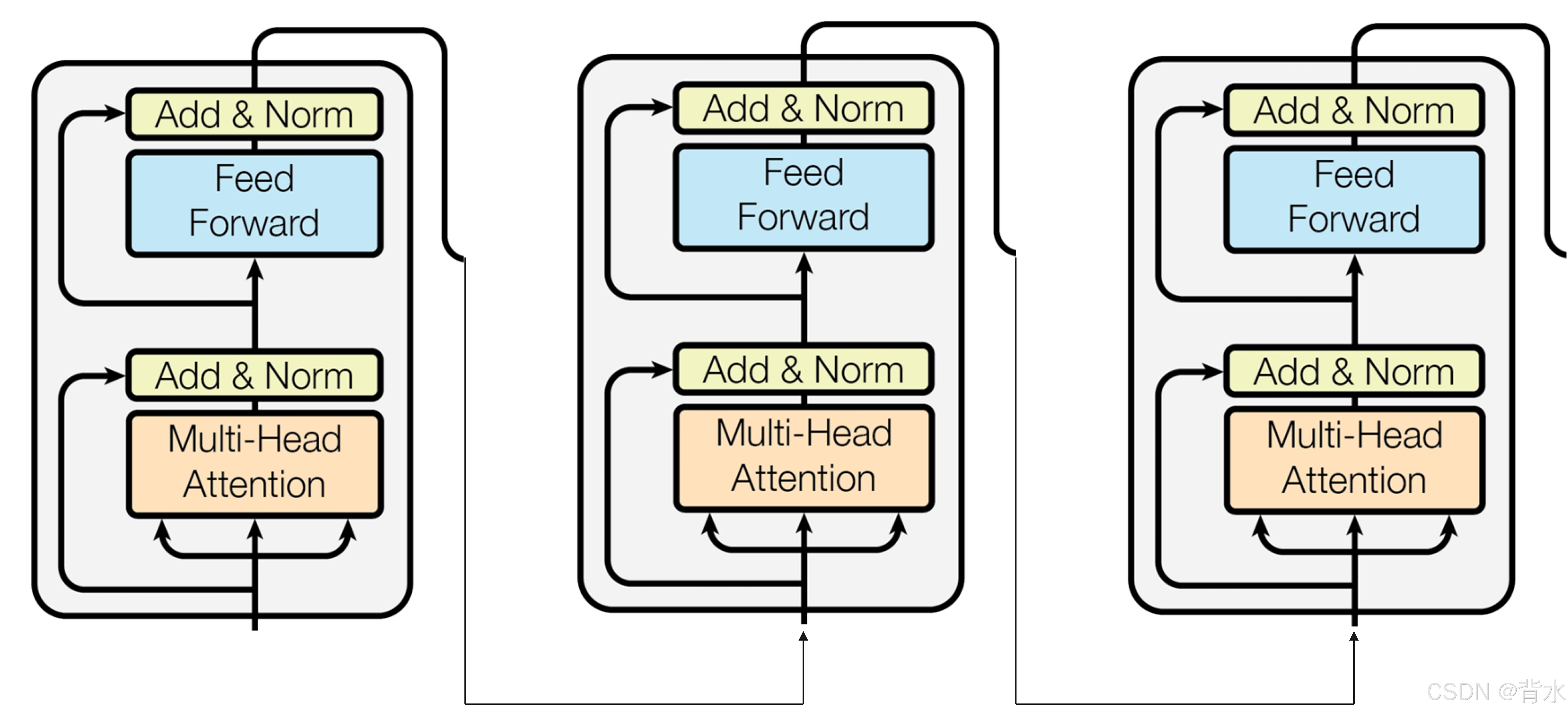
解码器部分层和层之间的连接
2.8.1. 解码层实现
class DecoderLayer(nn.Module):
    def __init__(self, size, self_attn, src_attn, feed_forward, dropout):
        super(DecoderLayer, self).__init__()
        self.size = size
        self.self_attn = self_attn  # 掩码的自注意力机制对象
        self.src_attn = src_attn  # encode-decoder注意力机制对象
        self.feed_forward = feed_forward
        self.sublayer = clones(SublayerConnection(size, dropout), 3)

    def forward(self, x, memory, source_mask, target_mask):
        m = memory
        x = self.sublayer[0](x, lambda x: self.self_attn(x, x, x, target_mask))
        x = self.sublayer[1](x, lambda x: self.src_attn(x, m, m, source_mask))
        x = self.sublayer[2](x, self.feed_forward)

        return x


def test_DecoderLayer():
    # 准备数据
    pe_result = torch.randn(2, 4, 512)

    # 实例化多头注意力机制对象
    source_mask = Variable(torch.zeros(8, 4, 4))
    target_mask = Variable(torch.zeros(8, 4, 4))
    self_attn = src_attn = MultiHeadedAttention(8, 512, 0.1)

    # 实例化PositionwiseFeedForward
    d_model, d_ff = 512, 1024
    ff = PositionwiseFeedForward(d_model, d_ff)

    # 实例化 一个 编码器层
    my_decoderlayer = DecoderLayer(512, self_attn, src_attn, ff, 0.1)
    print('my_decoderlayer--->', my_decoderlayer)

    # 准备编码器部分的最后编码结果 也就是中间语义张量C
    memory = torch.randn(2, 4, 512)

    dl_result = my_decoderlayer(pe_result, memory, source_mask, target_mask)
    print('dl_result--->', dl_result.shape, dl_result)
运行结果:
my_decoderlayer---> DecoderLayer(
  (self_attn): MultiHeadedAttention(
    (linearList): ModuleList(
      (0): Linear(in_features=512, out_features=512, bias=True)
      (1): Linear(in_features=512, out_features=512, bias=True)
      (2): Linear(in_features=512, out_features=512, bias=True)
      (3): Linear(in_features=512, out_features=512, bias=True)
    )
    (dropout): Dropout(p=0.1, inplace=False)
  )
  (src_attn): MultiHeadedAttention(
    (linearList): ModuleList(
      (0): Linear(in_features=512, out_features=512, bias=True)
      (1): Linear(in_features=512, out_features=512, bias=True)
      (2): Linear(in_features=512, out_features=512, bias=True)
      (3): Linear(in_features=512, out_features=512, bias=True)
    )
    (dropout): Dropout(p=0.1, inplace=False)
  )
  (feed_forward): PositionwiseFeedForward(
    (w1): Linear(in_features=512, out_features=1024, bias=True)
    (w2): Linear(in_features=1024, out_features=512, bias=True)
    (dropout): Dropout(p=0.1, inplace=False)
  )
  (sublayer): ModuleList(
    (0): SublayerConnection(
      (norm): LayerNorm()
      (dropout): Dropout(p=0.1, inplace=False)
    )
    (1): SublayerConnection(
      (norm): LayerNorm()
      (dropout): Dropout(p=0.1, inplace=False)
    )
    (2): SublayerConnection(
      (norm): LayerNorm()
      (dropout): Dropout(p=0.1, inplace=False)
    )
  )
)
dl_result---> torch.Size([2, 4, 512]) tensor([[[-1.9936, -0.0402, -0.1751,  ..., -0.6314,  3.2067, -0.3326],
         [ 1.9374, -3.0052,  0.2525,  ...,  0.1920,  0.3456,  0.4651],
         [-0.5417,  0.2503, -1.2825,  ...,  0.1409,  1.1456, -0.7702],
         [-2.2342,  0.7363,  0.4629,  ...,  1.0374, -0.9062, -1.1992]],

        [[ 0.5788,  1.5665,  0.8883,  ...,  2.2583,  1.6104,  0.9706],
         [ 0.3898, -0.3707,  1.9917,  ..., -0.6044, -1.1714,  1.5677],
         [ 1.9121,  0.3596, -0.0594,  ..., -1.8380,  0.1604, -0.1955],
         [ 2.5033, -1.8340, -0.4194,  ..., -0.7945,  1.4294,  0.2188]]],
       grad_fn=<AddBackward0>)
2.8.2. 解码器实现
class Decoder(nn.Module):
    def __init__(self, layer, N):
        super(Decoder, self).__init__()
        self.layers = clones(layer, N)
        self.norm = LayerNorm(layer.size)

    def forward(self, x, memory, source_mask, target_mask):
        for layer in self.layers:
            x = layer(x, memory, source_mask, target_mask)

        x = self.norm(x)
        return x


def test_Decoder():
    c = copy.deepcopy

    # 准备数据
    pe_result = torch.randn(2, 4, 512)

    # 实例化多头注意力机制对象
    source_mask = Variable(torch.zeros(8, 4, 4))
    target_mask = Variable(torch.zeros(8, 4, 4))
    self_attn = src_attn = MultiHeadedAttention(8, 512, 0.1)

    # 实例化PositionwiseFeedForward
    d_model, d_ff = 512, 1024
    ff = PositionwiseFeedForward(d_model, d_ff)

    # 实例化 一个 编码器层
    my_decoderlayer = DecoderLayer(512, c(self_attn), c(src_attn), c(ff), 0.1)
    # print('my_decoderlayer--->', my_decoderlayer)

    # # 准备编码器部分的最后编码结果 也就是中间语义张量C
    memory = torch.randn(2, 4, 512)

    # 实例化解码器部分
    my_decoder = Decoder(my_decoderlayer, 3)
    print('my_decoder--->', my_decoder)

    # 让数据经过解码器部分
    decoder_result = my_decoder(pe_result, memory, source_mask, target_mask)
    print('decoder_result--->', decoder_result.shape, decoder_result)
运行结果:
my_decoder---> Decoder(
  (layers): ModuleList(
    (0): DecoderLayer(
      (self_attn): MultiHeadedAttention(
        (linearList): ModuleList(
          (0): Linear(in_features=512, out_features=512, bias=True)
          (1): Linear(in_features=512, out_features=512, bias=True)
          (2): Linear(in_features=512, out_features=512, bias=True)
          (3): Linear(in_features=512, out_features=512, bias=True)
        )
        (dropout): Dropout(p=0.1, inplace=False)
      )
      (src_attn): MultiHeadedAttention(
        (linearList): ModuleList(
          (0): Linear(in_features=512, out_features=512, bias=True)
          (1): Linear(in_features=512, out_features=512, bias=True)
          (2): Linear(in_features=512, out_features=512, bias=True)
          (3): Linear(in_features=512, out_features=512, bias=True)
        )
        (dropout): Dropout(p=0.1, inplace=False)
      )
      (feed_forward): PositionwiseFeedForward(
        (w1): Linear(in_features=512, out_features=1024, bias=True)
        (w2): Linear(in_features=1024, out_features=512, bias=True)
        (dropout): Dropout(p=0.1, inplace=False)
      )
      (sublayer): ModuleList(
        (0): SublayerConnection(
          (norm): LayerNorm()
          (dropout): Dropout(p=0.1, inplace=False)
        )
        (1): SublayerConnection(
          (norm): LayerNorm()
          (dropout): Dropout(p=0.1, inplace=False)
        )
        (2): SublayerConnection(
          (norm): LayerNorm()
          (dropout): Dropout(p=0.1, inplace=False)
        )
      )
    )
    (1): DecoderLayer(
      (self_attn): MultiHeadedAttention(
        (linearList): ModuleList(
          (0): Linear(in_features=512, out_features=512, bias=True)
          (1): Linear(in_features=512, out_features=512, bias=True)
          (2): Linear(in_features=512, out_features=512, bias=True)
          (3): Linear(in_features=512, out_features=512, bias=True)
        )
        (dropout): Dropout(p=0.1, inplace=False)
      )
      (src_attn): MultiHeadedAttention(
        (linearList): ModuleList(
          (0): Linear(in_features=512, out_features=512, bias=True)
          (1): Linear(in_features=512, out_features=512, bias=True)
          (2): Linear(in_features=512, out_features=512, bias=True)
          (3): Linear(in_features=512, out_features=512, bias=True)
        )
        (dropout): Dropout(p=0.1, inplace=False)
      )
      (feed_forward): PositionwiseFeedForward(
        (w1): Linear(in_features=512, out_features=1024, bias=True)
        (w2): Linear(in_features=1024, out_features=512, bias=True)
        (dropout): Dropout(p=0.1, inplace=False)
      )
      (sublayer): ModuleList(
        (0): SublayerConnection(
          (norm): LayerNorm()
          (dropout): Dropout(p=0.1, inplace=False)
        )
        (1): SublayerConnection(
          (norm): LayerNorm()
          (dropout): Dropout(p=0.1, inplace=False)
        )
        (2): SublayerConnection(
          (norm): LayerNorm()
          (dropout): Dropout(p=0.1, inplace=False)
        )
      )
    )
    (2): DecoderLayer(
      (self_attn): MultiHeadedAttention(
        (linearList): ModuleList(
          (0): Linear(in_features=512, out_features=512, bias=True)
          (1): Linear(in_features=512, out_features=512, bias=True)
          (2): Linear(in_features=512, out_features=512, bias=True)
          (3): Linear(in_features=512, out_features=512, bias=True)
        )
        (dropout): Dropout(p=0.1, inplace=False)
      )
      (src_attn): MultiHeadedAttention(
        (linearList): ModuleList(
          (0): Linear(in_features=512, out_features=512, bias=True)
          (1): Linear(in_features=512, out_features=512, bias=True)
          (2): Linear(in_features=512, out_features=512, bias=True)
          (3): Linear(in_features=512, out_features=512, bias=True)
        )
        (dropout): Dropout(p=0.1, inplace=False)
      )
      (feed_forward): PositionwiseFeedForward(
        (w1): Linear(in_features=512, out_features=1024, bias=True)
        (w2): Linear(in_features=1024, out_features=512, bias=True)
        (dropout): Dropout(p=0.1, inplace=False)
      )
      (sublayer): ModuleList(
        (0): SublayerConnection(
          (norm): LayerNorm()
          (dropout): Dropout(p=0.1, inplace=False)
        )
        (1): SublayerConnection(
          (norm): LayerNorm()
          (dropout): Dropout(p=0.1, inplace=False)
        )
        (2): SublayerConnection(
          (norm): LayerNorm()
          (dropout): Dropout(p=0.1, inplace=False)
        )
      )
    )
  )
  (norm): LayerNorm()
)
decoder_result---> torch.Size([2, 4, 512]) tensor([[[ 1.4851,  0.4897,  1.0998,  ..., -0.1003, -0.2074, -0.5833],
         [ 1.0350,  0.3608,  0.8961,  ...,  0.0074,  1.2578,  0.4501],
         [ 0.6086, -0.1170,  1.4844,  ...,  0.0086,  1.2520,  0.3547],
         [ 1.0239,  0.6110,  0.6716,  ..., -0.8469,  0.1217,  0.0685]],

        [[ 0.0459, -1.0399,  0.6293,  ..., -0.0794,  0.2749, -0.6378],
         [-0.1149,  0.9141,  1.8580,  ..., -0.2664,  1.0761, -0.4101],
         [-0.2547,  1.2553,  0.8377,  ..., -1.4234,  1.1622, -0.6038],
         [ 0.9534,  0.9458,  0.8968,  ..., -0.5697,  0.1892,  0.1908]]],
       grad_fn=<AddBackward0>)
完结
如有错误或者不足,请在评论区指正!