- 🍨 本文为🔗365天深度学习训练营 中的学习记录博客
- 🍖 原作者:K同学啊 | 接辅导、项目定制
一、我的环境:
1.语言环境:Python 3.9
2.编译器:Pycharm
3.深度学习环境:
- torch==2.1.2+cu118
- torchvision==0.16.2+cu118
二、GPU设置:
import torch

device = torch.device("cuda" if torch.cuda.is_available() else "cpu")
print(device)三、导入数据:
- pathlib.Path函数将字符串类型的文件夹路径转换为pathlib.Path对象。
- glob()方法获取data_dir路径下的所有文件路径,并以列表形式存储在data_paths中。
- split()函数对data_paths中的每个文件路径执行分割操作,获得各个文件所属的类别名称,并存储在classeNames中。
- 打印classeNames列表,显示每个文件所属的类别名称
data_dir = './data/weather_photos/'
data_dir = pathlib.Path(data_dir)

data_paths = list(data_dir.glob('*'))
classeNames = [str(path).split("\\")[1] for path in data_paths]
print(classeNames)
运行结果:
['cloudy', 'rain', 'shine', 'sunrise']total_datadir = './data/weather_photos'
# 关于transforms.Compose的更多介绍可以参考:https://blog.csdn.net/qq_38251616/article/details/124878863
train_transforms = transforms.Compose([
transforms.Resize([224, 224]), # 将输入图片resize成统一尺寸
transforms.ToTensor(), # 将PIL Image或numpy.ndarray转换为tensor,并归一化到[0,1]之间
transforms.Normalize( # 标准化处理-->转换为标准正太分布(高斯分布),使模型更容易收敛
mean=[0.485, 0.456, 0.406],
std=[0.229, 0.224, 0.225]) # 其中 mean=[0.485,0.456,0.406]与std=[0.229,0.224,0.225] 从数据集中随机抽样计算得到的。
])
total_data = datasets.ImageFolder(total_datadir,transform=train_transforms)
print(total_data)运行结果:
Dataset ImageFolder
    Number of datapoints: 1125
    Root location: ./data/weather_photos
    StandardTransform
Transform: Compose(
               Resize(size=[224, 224], interpolation=bilinear, max_size=None, antialias=True)
               ToTensor()
               Normalize(mean=[0.485, 0.456, 0.406], std=[0.229, 0.224, 0.225])
)四、数据可视化:
import matplotlib.pyplot as plt
from PIL import Image

# 指定图像文件夹路径
image_folder = './data/weather_photos/cloudy/'

# 获取文件夹中的所有图像文件
image_files = [f for f in os.listdir(image_folder) if f.endswith((".jpg", ".png", ".jpeg"))]

# 创建Matplotlib图像
fig, axes = plt.subplots(3, 8, figsize=(16, 6))

# 使用列表推导式加载和显示图像
for ax, img_file in zip(axes.flat, image_files):
    img_path = os.path.join(image_folder, img_file)
    img = Image.open(img_path)
    ax.imshow(img)
    ax.axis('off')

# 显示图像
plt.tight_layout()
plt.show()
运行结果:

五、划分数据集
train_size = int(0.8 * len(total_data))
test_size  = len(total_data) - train_size
train_dataset, test_dataset = torch.utils.data.random_split(total_data, [train_size, test_size])
print(train_size,test_size)
batch_size = 4
train_dl = torch.utils.data.DataLoader(train_dataset,
batch_size=batch_size,
shuffle=True,
num_workers=1)
test_dl = torch.utils.data.DataLoader(test_dataset,
batch_size=batch_size,
shuffle=True,
num_workers=1)for X, y in test_dl:
print("Shape of X [N, C, H, W]: ", X.shape)
print("Shape of y: ", y.shape, y.dtype)
break运行结果:
Shape of X [N, C, H, W]:  torch.Size([4, 3, 224, 224])
Shape of y:  torch.Size([4]) torch.int64
六、搭建包含Backbone模块的模型
def autopad(k, p=None):  # kernel, padding
    # Pad to 'same'
    if p is None:
        p = k // 2 if isinstance(k, int) else [x // 2 for x in k]  # auto-pad
    return p

class Conv(nn.Module):
    # Standard convolution
    def __init__(self, c1, c2, k=1, s=1, p=None, g=1, act=True):  # ch_in, ch_out, kernel, stride, padding, groups
        super().__init__()
        self.conv = nn.Conv2d(c1, c2, k, s, autopad(k, p), groups=g, bias=False)
        self.bn = nn.BatchNorm2d(c2)
        self.act = nn.SiLU() if act is True else (act if isinstance(act, nn.Module) else nn.Identity())

    def forward(self, x):
        return self.act(self.bn(self.conv(x)))

class Bottleneck(nn.Module):
    # Standard bottleneck
    def __init__(self, c1, c2, shortcut=True, g=1, e=0.5):  # ch_in, ch_out, shortcut, groups, expansion
        super().__init__()
        c_ = int(c2 * e)  # hidden channels
        self.cv1 = Conv(c1, c_, 1, 1)
        self.cv2 = Conv(c_, c2, 3, 1, g=g)
        self.add = shortcut and c1 == c2

    def forward(self, x):
        return x + self.cv2(self.cv1(x)) if self.add else self.cv2(self.cv1(x))

class C3(nn.Module):
    # CSP Bottleneck with 3 convolutions
    def __init__(self, c1, c2, n=1, shortcut=True, g=1, e=0.5):  # ch_in, ch_out, number, shortcut, groups, expansion
        super().__init__()
        c_ = int(c2 * e)  # hidden channels
        self.cv1 = Conv(c1, c_, 1, 1)
        self.cv2 = Conv(c1, c_, 1, 1)
        self.cv3 = Conv(2 * c_, c2, 1)  # act=FReLU(c2)
        self.m = nn.Sequential(*(Bottleneck(c_, c_, shortcut, g, e=1.0) for _ in range(n)))

    def forward(self, x):
        return self.cv3(torch.cat((self.m(self.cv1(x)), self.cv2(x)), dim=1))

class SPPF(nn.Module):
    # Spatial Pyramid Pooling - Fast (SPPF) layer for YOLOv5 by Glenn Jocher
    def __init__(self, c1, c2, k=5):  # equivalent to SPP(k=(5, 9, 13))
        super().__init__()
        c_ = c1 // 2  # hidden channels
        self.cv1 = Conv(c1, c_, 1, 1)
        self.cv2 = Conv(c_ * 4, c2, 1, 1)
        self.m = nn.MaxPool2d(kernel_size=k, stride=1, padding=k // 2)

    def forward(self, x):
        x = self.cv1(x)
        with warnings.catch_warnings():
            warnings.simplefilter('ignore')  # suppress torch 1.9.0 max_pool2d() warning
            y1 = self.m(x)
            y2 = self.m(y1)
            return self.cv2(torch.cat([x, y1, y2, self.m(y2)], 1))
"""
这个是YOLOv5, 6.0版本的主干网络,这里进行复现
(注:有部分删改,详细讲解将在后续进行展开)
"""
class YOLOv5_backbone(nn.Module):
    def __init__(self):
        super(YOLOv5_backbone, self).__init__()

        self.Conv_1 = Conv(3, 64, 3, 2, 2)
        self.Conv_2 = Conv(64, 128, 3, 2)
        self.C3_3   = C3(128,128)
        self.Conv_4 = Conv(128, 256, 3, 2)
        self.C3_5   = C3(256,256)
        self.Conv_6 = Conv(256, 512, 3, 2)
        self.C3_7   = C3(512,512)
        self.Conv_8 = Conv(512, 1024, 3, 2)
        self.C3_9   = C3(1024, 1024)
        self.SPPF   = SPPF(1024, 1024, 5)

        # 全连接网络层,用于分类
        self.classifier = nn.Sequential(
            nn.Linear(in_features=65536, out_features=100),
            nn.ReLU(),
            nn.Linear(in_features=100, out_features=4)
        )

    def forward(self, x):
        x = self.Conv_1(x)
        x = self.Conv_2(x)
        x = self.C3_3(x)
        x = self.Conv_4(x)
        x = self.C3_5(x)
        x = self.Conv_6(x)
        x = self.C3_7(x)
        x = self.Conv_8(x)
        x = self.C3_9(x)
        x = self.SPPF(x)

        x = torch.flatten(x, start_dim=1)
        x = self.classifier(x)

        return x
加载并打印模型
import torchsummary as summary

model = YOLOv5_backbone()
summary.summary(model, (3, 224, 224))
运行结果:
----------------------------------------------------------------
        Layer (type)               Output Shape         Param #
================================================================
            Conv2d-1         [-1, 64, 113, 113]           1,728
       BatchNorm2d-2         [-1, 64, 113, 113]             128
              SiLU-3         [-1, 64, 113, 113]               0
              Conv-4         [-1, 64, 113, 113]               0
            Conv2d-5          [-1, 128, 57, 57]          73,728
       BatchNorm2d-6          [-1, 128, 57, 57]             256
              SiLU-7          [-1, 128, 57, 57]               0
              Conv-8          [-1, 128, 57, 57]               0
            Conv2d-9           [-1, 64, 57, 57]           8,192
      BatchNorm2d-10           [-1, 64, 57, 57]             128
             SiLU-11           [-1, 64, 57, 57]               0
             Conv-12           [-1, 64, 57, 57]               0
           Conv2d-13           [-1, 64, 57, 57]           4,096
      BatchNorm2d-14           [-1, 64, 57, 57]             128
             SiLU-15           [-1, 64, 57, 57]               0
             Conv-16           [-1, 64, 57, 57]               0
           Conv2d-17           [-1, 64, 57, 57]          36,864
      BatchNorm2d-18           [-1, 64, 57, 57]             128
             SiLU-19           [-1, 64, 57, 57]               0
             Conv-20           [-1, 64, 57, 57]               0
       Bottleneck-21           [-1, 64, 57, 57]               0
           Conv2d-22           [-1, 64, 57, 57]           8,192
      BatchNorm2d-23           [-1, 64, 57, 57]             128
             SiLU-24           [-1, 64, 57, 57]               0
             Conv-25           [-1, 64, 57, 57]               0
           Conv2d-26          [-1, 128, 57, 57]          16,384
      BatchNorm2d-27          [-1, 128, 57, 57]             256
             SiLU-28          [-1, 128, 57, 57]               0
             Conv-29          [-1, 128, 57, 57]               0
               C3-30          [-1, 128, 57, 57]               0
           Conv2d-31          [-1, 256, 29, 29]         294,912
      BatchNorm2d-32          [-1, 256, 29, 29]             512
             SiLU-33          [-1, 256, 29, 29]               0
             Conv-34          [-1, 256, 29, 29]               0
           Conv2d-35          [-1, 128, 29, 29]          32,768
      BatchNorm2d-36          [-1, 128, 29, 29]             256
             SiLU-37          [-1, 128, 29, 29]               0
             Conv-38          [-1, 128, 29, 29]               0
           Conv2d-39          [-1, 128, 29, 29]          16,384
      BatchNorm2d-40          [-1, 128, 29, 29]             256
             SiLU-41          [-1, 128, 29, 29]               0
             Conv-42          [-1, 128, 29, 29]               0
           Conv2d-43          [-1, 128, 29, 29]         147,456
      BatchNorm2d-44          [-1, 128, 29, 29]             256
             SiLU-45          [-1, 128, 29, 29]               0
             Conv-46          [-1, 128, 29, 29]               0
       Bottleneck-47          [-1, 128, 29, 29]               0
           Conv2d-48          [-1, 128, 29, 29]          32,768
      BatchNorm2d-49          [-1, 128, 29, 29]             256
             SiLU-50          [-1, 128, 29, 29]               0
             Conv-51          [-1, 128, 29, 29]               0
           Conv2d-52          [-1, 256, 29, 29]          65,536
      BatchNorm2d-53          [-1, 256, 29, 29]             512
             SiLU-54          [-1, 256, 29, 29]               0
             Conv-55          [-1, 256, 29, 29]               0
               C3-56          [-1, 256, 29, 29]               0
           Conv2d-57          [-1, 512, 15, 15]       1,179,648
      BatchNorm2d-58          [-1, 512, 15, 15]           1,024
             SiLU-59          [-1, 512, 15, 15]               0
             Conv-60          [-1, 512, 15, 15]               0
           Conv2d-61          [-1, 256, 15, 15]         131,072
      BatchNorm2d-62          [-1, 256, 15, 15]             512
             SiLU-63          [-1, 256, 15, 15]               0
             Conv-64          [-1, 256, 15, 15]               0
           Conv2d-65          [-1, 256, 15, 15]          65,536
      BatchNorm2d-66          [-1, 256, 15, 15]             512
             SiLU-67          [-1, 256, 15, 15]               0
             Conv-68          [-1, 256, 15, 15]               0
           Conv2d-69          [-1, 256, 15, 15]         589,824
      BatchNorm2d-70          [-1, 256, 15, 15]             512
             SiLU-71          [-1, 256, 15, 15]               0
             Conv-72          [-1, 256, 15, 15]               0
       Bottleneck-73          [-1, 256, 15, 15]               0
           Conv2d-74          [-1, 256, 15, 15]         131,072
      BatchNorm2d-75          [-1, 256, 15, 15]             512
             SiLU-76          [-1, 256, 15, 15]               0
             Conv-77          [-1, 256, 15, 15]               0
           Conv2d-78          [-1, 512, 15, 15]         262,144
      BatchNorm2d-79          [-1, 512, 15, 15]           1,024
             SiLU-80          [-1, 512, 15, 15]               0
             Conv-81          [-1, 512, 15, 15]               0
               C3-82          [-1, 512, 15, 15]               0
           Conv2d-83           [-1, 1024, 8, 8]       4,718,592
      BatchNorm2d-84           [-1, 1024, 8, 8]           2,048
             SiLU-85           [-1, 1024, 8, 8]               0
             Conv-86           [-1, 1024, 8, 8]               0
           Conv2d-87            [-1, 512, 8, 8]         524,288
      BatchNorm2d-88            [-1, 512, 8, 8]           1,024
             SiLU-89            [-1, 512, 8, 8]               0
             Conv-90            [-1, 512, 8, 8]               0
           Conv2d-91            [-1, 512, 8, 8]         262,144
      BatchNorm2d-92            [-1, 512, 8, 8]           1,024
             SiLU-93            [-1, 512, 8, 8]               0
             Conv-94            [-1, 512, 8, 8]               0
           Conv2d-95            [-1, 512, 8, 8]       2,359,296
      BatchNorm2d-96            [-1, 512, 8, 8]           1,024
             SiLU-97            [-1, 512, 8, 8]               0
             Conv-98            [-1, 512, 8, 8]               0
       Bottleneck-99            [-1, 512, 8, 8]               0
          Conv2d-100            [-1, 512, 8, 8]         524,288
     BatchNorm2d-101            [-1, 512, 8, 8]           1,024
            SiLU-102            [-1, 512, 8, 8]               0
            Conv-103            [-1, 512, 8, 8]               0
          Conv2d-104           [-1, 1024, 8, 8]       1,048,576
     BatchNorm2d-105           [-1, 1024, 8, 8]           2,048
            SiLU-106           [-1, 1024, 8, 8]               0
            Conv-107           [-1, 1024, 8, 8]               0
              C3-108           [-1, 1024, 8, 8]               0
          Conv2d-109            [-1, 512, 8, 8]         524,288
     BatchNorm2d-110            [-1, 512, 8, 8]           1,024
            SiLU-111            [-1, 512, 8, 8]               0
            Conv-112            [-1, 512, 8, 8]               0
       MaxPool2d-113            [-1, 512, 8, 8]               0
       MaxPool2d-114            [-1, 512, 8, 8]               0
       MaxPool2d-115            [-1, 512, 8, 8]               0
          Conv2d-116           [-1, 1024, 8, 8]       2,097,152
     BatchNorm2d-117           [-1, 1024, 8, 8]           2,048
            SiLU-118           [-1, 1024, 8, 8]               0
            Conv-119           [-1, 1024, 8, 8]               0
            SPPF-120           [-1, 1024, 8, 8]               0
          Linear-121                  [-1, 100]       6,553,700
            ReLU-122                  [-1, 100]               0
          Linear-123                    [-1, 4]             404
================================================================
Total params: 21,729,592
Trainable params: 21,729,592
Non-trainable params: 0
----------------------------------------------------------------
Input size (MB): 0.57
Forward/backward pass size (MB): 137.59
Params size (MB): 82.89
Estimated Total Size (MB): 221.06
----------------------------------------------------------------
七、训练函数
# 训练循环
def train(dataloader, model, loss_fn, optimizer):
    size = len(dataloader.dataset)  # 训练集的大小
    num_batches = len(dataloader)   # 批次数目, (size/batch_size,向上取整)

    train_loss, train_acc = 0, 0  # 初始化训练损失和正确率

    for X, y in dataloader:  # 获取图片及其标签
        X, y = X.to(device), y.to(device)

        # 计算预测误差
        pred = model(X)          # 网络输出
        loss = loss_fn(pred, y)  # 计算网络输出和真实值之间的差距,targets为真实值,计算二者差值即为损失

        # 反向传播
        optimizer.zero_grad()  # grad属性归零
        loss.backward()        # 反向传播
        optimizer.step()       # 每一步自动更新

        # 记录acc与loss
        train_acc  += (pred.argmax(1) == y).type(torch.float).sum().item()
        train_loss += loss.item()

    train_acc  /= size
    train_loss /= num_batches

    return train_acc, train_loss
八、测试函数
def test (dataloader, model, loss_fn):
    size        = len(dataloader.dataset)  # 测试集的大小
    num_batches = len(dataloader)          # 批次数目, (size/batch_size,向上取整)
    test_loss, test_acc = 0, 0

    # 当不进行训练时,停止梯度更新,节省计算内存消耗
    with torch.no_grad():
        for imgs, target in dataloader:
            imgs, target = imgs.to(device), target.to(device)

            # 计算loss
            target_pred = model(imgs)
            loss        = loss_fn(target_pred, target)

            test_loss += loss.item()
            test_acc  += (target_pred.argmax(1) == target).type(torch.float).sum().item()

    test_acc  /= size
    test_loss /= num_batches

    return test_acc, test_loss
九、模型训练
if __name__ == "__main__":
    main()
def main():
optimizer = torch.optim.Adam(model.parameters(), lr= 1e-4)
loss_fn = nn.CrossEntropyLoss() # 创建损失函数
epochs = 60
train_loss = []
train_acc = []
test_loss = []
test_acc = []
best_acc = 0 # 设置一个最佳准确率,作为最佳模型的判别指标
for epoch in range(epochs):
model.train()
epoch_train_acc, epoch_train_loss = train(train_dl, model, loss_fn, optimizer)
model.eval()
epoch_test_acc, epoch_test_loss = test(test_dl, model, loss_fn)
# 保存最佳模型到 best_model
if epoch_test_acc > best_acc:
best_acc = epoch_test_acc
best_model = copy.deepcopy(model)
train_acc.append(epoch_train_acc)
train_loss.append(epoch_train_loss)
test_acc.append(epoch_test_acc)
test_loss.append(epoch_test_loss)
# 获取当前的学习率
lr = optimizer.state_dict()['param_groups'][0]['lr']
template = ('Epoch:{:2d}, Train_acc:{:.1f}%, Train_loss:{:.3f}, Test_acc:{:.1f}%, Test_loss:{:.3f}, Lr:{:.2E}')
print(template.format(epoch+1, epoch_train_acc*100, epoch_train_loss,
epoch_test_acc*100, epoch_test_loss, lr))
# 保存最佳模型到文件中
PATH = './best_model.pth' # 保存的参数文件名
torch.save(best_model.state_dict(), PATH)
print('Done')运行结果:
Epoch: 1,duration:14516ms, Train_acc:51.9%, Train_loss:1.178, Test_acc:59.1%, Test_loss:0.938, Lr:1.00E-04
Epoch: 2,duration:11299ms, Train_acc:65.0%, Train_loss:0.848, Test_acc:68.9%, Test_loss:0.592, Lr:1.00E-04
Epoch: 3,duration:11242ms, Train_acc:66.0%, Train_loss:0.772, Test_acc:79.6%, Test_loss:0.455, Lr:1.00E-04
Epoch: 4,duration:11300ms, Train_acc:71.0%, Train_loss:0.701, Test_acc:71.6%, Test_loss:0.561, Lr:1.00E-04
Epoch: 5,duration:11248ms, Train_acc:75.8%, Train_loss:0.629, Test_acc:75.1%, Test_loss:0.633, Lr:1.00E-04
Epoch: 6,duration:11275ms, Train_acc:80.3%, Train_loss:0.512, Test_acc:83.1%, Test_loss:0.455, Lr:1.00E-04
Epoch: 7,duration:11172ms, Train_acc:82.3%, Train_loss:0.476, Test_acc:84.4%, Test_loss:0.377, Lr:1.00E-04
Epoch: 8,duration:11269ms, Train_acc:85.3%, Train_loss:0.392, Test_acc:82.2%, Test_loss:0.373, Lr:1.00E-04
Epoch: 9,duration:11182ms, Train_acc:86.3%, Train_loss:0.355, Test_acc:80.4%, Test_loss:0.505, Lr:1.00E-04
Epoch:10,duration:11316ms, Train_acc:89.2%, Train_loss:0.280, Test_acc:88.4%, Test_loss:0.253, Lr:1.00E-04
Epoch:11,duration:11279ms, Train_acc:86.0%, Train_loss:0.355, Test_acc:85.8%, Test_loss:0.307, Lr:1.00E-04
Epoch:12,duration:11366ms, Train_acc:88.4%, Train_loss:0.273, Test_acc:85.8%, Test_loss:0.311, Lr:1.00E-04
Epoch:13,duration:11298ms, Train_acc:91.6%, Train_loss:0.252, Test_acc:90.7%, Test_loss:0.253, Lr:1.00E-04
Epoch:14,duration:11232ms, Train_acc:92.6%, Train_loss:0.223, Test_acc:91.1%, Test_loss:0.259, Lr:1.00E-04
Epoch:15,duration:11270ms, Train_acc:90.6%, Train_loss:0.237, Test_acc:91.1%, Test_loss:0.308, Lr:1.00E-04
Epoch:16,duration:11526ms, Train_acc:92.9%, Train_loss:0.178, Test_acc:96.4%, Test_loss:0.118, Lr:1.00E-04
Epoch:17,duration:11227ms, Train_acc:95.9%, Train_loss:0.095, Test_acc:93.3%, Test_loss:0.192, Lr:1.00E-04
Epoch:18,duration:11386ms, Train_acc:96.7%, Train_loss:0.100, Test_acc:90.7%, Test_loss:0.285, Lr:1.00E-04
Epoch:19,duration:11311ms, Train_acc:93.7%, Train_loss:0.165, Test_acc:88.4%, Test_loss:0.318, Lr:1.00E-04
Epoch:20,duration:12990ms, Train_acc:95.4%, Train_loss:0.122, Test_acc:93.8%, Test_loss:0.175, Lr:1.00E-04
Epoch:21,duration:13676ms, Train_acc:98.2%, Train_loss:0.063, Test_acc:93.8%, Test_loss:0.224, Lr:1.00E-04
Epoch:22,duration:13579ms, Train_acc:95.8%, Train_loss:0.128, Test_acc:93.3%, Test_loss:0.216, Lr:1.00E-04
Epoch:23,duration:13570ms, Train_acc:97.9%, Train_loss:0.048, Test_acc:93.8%, Test_loss:0.159, Lr:1.00E-04
Epoch:24,duration:13574ms, Train_acc:97.2%, Train_loss:0.060, Test_acc:89.3%, Test_loss:0.332, Lr:1.00E-04
Epoch:25,duration:13452ms, Train_acc:96.4%, Train_loss:0.109, Test_acc:94.2%, Test_loss:0.168, Lr:1.00E-04
Epoch:26,duration:13688ms, Train_acc:95.0%, Train_loss:0.145, Test_acc:88.9%, Test_loss:0.378, Lr:1.00E-04
Epoch:27,duration:12939ms, Train_acc:97.8%, Train_loss:0.064, Test_acc:95.1%, Test_loss:0.125, Lr:1.00E-04
Epoch:28,duration:13189ms, Train_acc:99.0%, Train_loss:0.027, Test_acc:95.6%, Test_loss:0.094, Lr:1.00E-04
Epoch:29,duration:13725ms, Train_acc:98.2%, Train_loss:0.049, Test_acc:94.7%, Test_loss:0.116, Lr:1.00E-04
Epoch:30,duration:13993ms, Train_acc:96.3%, Train_loss:0.125, Test_acc:90.2%, Test_loss:0.374, Lr:1.00E-04
Epoch:31,duration:13697ms, Train_acc:95.8%, Train_loss:0.120, Test_acc:94.7%, Test_loss:0.168, Lr:1.00E-04
Epoch:32,duration:13256ms, Train_acc:97.3%, Train_loss:0.081, Test_acc:89.8%, Test_loss:0.320, Lr:1.00E-04
Epoch:33,duration:13659ms, Train_acc:97.8%, Train_loss:0.058, Test_acc:94.2%, Test_loss:0.203, Lr:1.00E-04
Epoch:34,duration:12981ms, Train_acc:98.2%, Train_loss:0.048, Test_acc:88.9%, Test_loss:0.302, Lr:1.00E-04
Epoch:35,duration:13278ms, Train_acc:98.0%, Train_loss:0.050, Test_acc:93.3%, Test_loss:0.180, Lr:1.00E-04
Epoch:36,duration:13643ms, Train_acc:98.6%, Train_loss:0.041, Test_acc:93.8%, Test_loss:0.215, Lr:1.00E-04
Epoch:37,duration:12959ms, Train_acc:99.4%, Train_loss:0.016, Test_acc:95.1%, Test_loss:0.135, Lr:1.00E-04
Epoch:38,duration:13252ms, Train_acc:99.4%, Train_loss:0.016, Test_acc:93.3%, Test_loss:0.239, Lr:1.00E-04
Epoch:39,duration:13256ms, Train_acc:96.7%, Train_loss:0.104, Test_acc:88.4%, Test_loss:0.414, Lr:1.00E-04
Epoch:40,duration:13169ms, Train_acc:97.7%, Train_loss:0.071, Test_acc:92.4%, Test_loss:0.220, Lr:1.00E-04
Epoch:41,duration:12490ms, Train_acc:99.2%, Train_loss:0.026, Test_acc:94.7%, Test_loss:0.138, Lr:1.00E-04
Epoch:42,duration:11181ms, Train_acc:98.7%, Train_loss:0.042, Test_acc:92.0%, Test_loss:0.246, Lr:1.00E-04
Epoch:43,duration:11210ms, Train_acc:98.8%, Train_loss:0.045, Test_acc:90.7%, Test_loss:0.299, Lr:1.00E-04
Epoch:44,duration:11399ms, Train_acc:99.1%, Train_loss:0.028, Test_acc:90.7%, Test_loss:0.316, Lr:1.00E-04
Epoch:45,duration:11255ms, Train_acc:97.6%, Train_loss:0.069, Test_acc:91.1%, Test_loss:0.251, Lr:1.00E-04
Epoch:46,duration:11540ms, Train_acc:98.4%, Train_loss:0.050, Test_acc:92.0%, Test_loss:0.282, Lr:1.00E-04
Epoch:47,duration:14299ms, Train_acc:97.7%, Train_loss:0.074, Test_acc:90.2%, Test_loss:0.289, Lr:1.00E-04
Epoch:48,duration:13733ms, Train_acc:98.2%, Train_loss:0.045, Test_acc:94.2%, Test_loss:0.196, Lr:1.00E-04
Epoch:49,duration:13832ms, Train_acc:98.8%, Train_loss:0.029, Test_acc:92.4%, Test_loss:0.248, Lr:1.00E-04
Epoch:50,duration:13235ms, Train_acc:98.9%, Train_loss:0.029, Test_acc:93.8%, Test_loss:0.182, Lr:1.00E-04
Epoch:51,duration:13804ms, Train_acc:99.0%, Train_loss:0.030, Test_acc:89.3%, Test_loss:0.328, Lr:1.00E-04
Epoch:52,duration:13920ms, Train_acc:98.2%, Train_loss:0.045, Test_acc:91.6%, Test_loss:0.235, Lr:1.00E-04
Epoch:53,duration:14425ms, Train_acc:99.1%, Train_loss:0.021, Test_acc:84.9%, Test_loss:0.693, Lr:1.00E-04
Epoch:54,duration:14777ms, Train_acc:97.0%, Train_loss:0.109, Test_acc:88.4%, Test_loss:0.540, Lr:1.00E-04
Epoch:55,duration:14075ms, Train_acc:97.4%, Train_loss:0.067, Test_acc:89.8%, Test_loss:0.365, Lr:1.00E-04
Epoch:56,duration:13698ms, Train_acc:99.4%, Train_loss:0.016, Test_acc:91.6%, Test_loss:0.337, Lr:1.00E-04
Epoch:57,duration:13465ms, Train_acc:98.7%, Train_loss:0.040, Test_acc:96.0%, Test_loss:0.189, Lr:1.00E-04
Epoch:58,duration:14171ms, Train_acc:99.0%, Train_loss:0.028, Test_acc:91.6%, Test_loss:0.208, Lr:1.00E-04
Epoch:59,duration:13446ms, Train_acc:99.9%, Train_loss:0.009, Test_acc:93.8%, Test_loss:0.213, Lr:1.00E-04
Epoch:60,duration:13758ms, Train_acc:98.7%, Train_loss:0.042, Test_acc:95.1%, Test_loss:0.160, Lr:1.00E-04
Done
十、模型评估
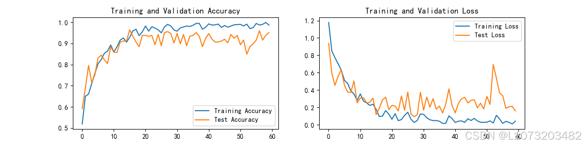
epochs_range = range(epochs)

plt.figure(figsize=(12, 3))
plt.subplot(1, 2, 1)

plt.plot(epochs_range, train_acc, label='Training Accuracy')
plt.plot(epochs_range, test_acc, label='Test Accuracy')
plt.legend(loc='lower right')
plt.title('Training and Validation Accuracy')

plt.subplot(1, 2, 2)
plt.plot(epochs_range, train_loss, label='Training Loss')
plt.plot(epochs_range, test_loss, label='Test Loss')
plt.legend(loc='upper right')
plt.title('Training and Validation Loss')
plt.show()
运行结果:
best_model.eval()
epoch_test_acc, epoch_test_loss = test(test_dl, best_model, loss_fn)
print(epoch_test_acc, epoch_test_loss)
0.9644444444444444 0.11823589946288848# 查看是否与我们记录的最高准确率一致
print(epoch_test_acc) #0.9644444444444444十一、总结
本次基于深度学习的pytorch实现YOLOv5-Backbone模块实现项目总结如下:
Backbone骨干网络
骨干网络是指用来提取图像特征的网络,它的主要作用是将原始的输入图像转化为多层特征图,以便后续的目标检测任务使用。在Yolov5中,使用的是CSPDarknet53或ResNet骨干网络,这两个网络都是相对轻量级的,能够在保证较高检测精度的同时,尽可能地减少计算量和内存占用。
Backbone中的主要结构有Conv模块、C3模块、SPPF模块。
Conv模块
Conv模块是卷积神经网络中常用的一种基础模块,它主要由卷积层、BN层和激活函数组成。下面对这些组成部分进行详细解析。

- 卷积层是卷积神经网络中最基础的层之一,用于提取输入特征中的局部空间信息。卷积操作可以看作是一个滑动窗口,窗口在输入特征上滑动,并将窗口内的特征值与卷积核进行卷积操作,从而得到输出特征。卷积层通常由多个卷积核组成,每个卷积核对应一个输出通道。卷积核的大小、步长、填充方式等超参数决定了卷积层的输出大小和感受野大小。卷积神经网络中,卷积层通常被用来构建特征提取器。
- BN层是在卷积层之后加入的一种归一化层,用于规范化神经网络中的特征值分布。它可以加速训练过程,提高模型泛化能力,减轻模型对初始化的依赖性。BN层的输入为一个batch的特征图,它将每个通道上的特征进行均值和方差的计算,并对每个通道上的特征进行标准化处理。标准化后的特征再通过一个可学习的仿射变换(拉伸和偏移)进行还原,从而得到BN层的输出。
- 激活函数是一种非线性函数,用于给神经网络引入非线性变换能力。常用的激活函数包括sigmoid、ReLU、LeakyReLU、ELU等。它们在输入值的不同范围内都有不同的输出表现,可以更好地适应不同类型的数据分布。
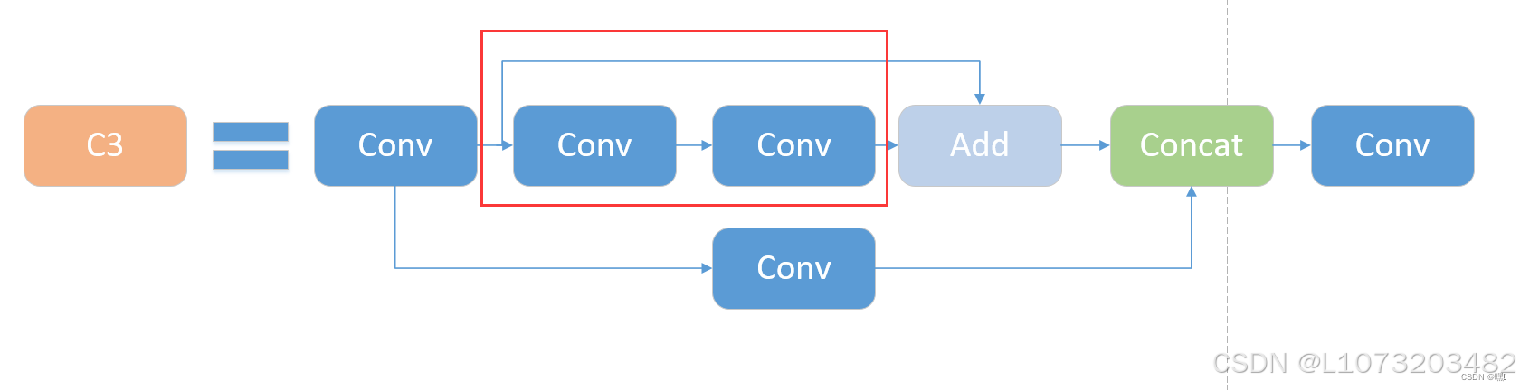
C3模块
C3模块是YOLOv5网络中的一个重要组成部分,其主要作用是增加网络的深度和感受野,提高特征提取的能力。
C3模块是由三个Conv块构成的,其中第一个Conv块的步幅为2,可以将特征图的尺寸减半,第二个Conv块和第三个Conv块的步幅为1。C3模块中的Conv块采用的都是3x3的卷积核。在每个Conv块之间,还加入了BN层和LeakyReLU激活函数,以提高模型的稳定性和泛化性能。
C3模块中的第一个Conv块的步幅为2,红色方框内两个Conv组成Bottleneck,这意味着它会将特征图的尺寸减半。这样做的目的是为了增加网络的感受野,同时减少计算量。通过将特征图的尺寸减半,可以使网络更加关注物体的全局信息,从而提高特征提取的效果。
C3模块中的第二个Conv块和第三个Conv块的步幅为1,这意味着它们不会改变特征图的尺寸。这样做的目的是为了保持特征图的空间分辨率,从而更好地保留物体的局部信息。同时,这两个Conv块的主要作用是进一步提取特征,增加网络的深度和感受野。
SPP
SPP模块是一种池化模块,通常应用于卷积神经网络中,旨在实现输入数据的空间不变性和位置不变性,以便于提高神经网络的识别能力。其主要思想是将不同大小的感受野应用于同一张图像,从而能够捕捉到不同尺度的特征信息。在SPP模块中,首先对输入特征图进行不同大小的池化操作,以得到一组不同大小的特征图。然后将这些特征图连接在一起,并通过全连接层进行降维,最终得到固定大小的特征向量。

SPP模块通常由三个步骤组成:
- 池化:将输入特征图分别进行不同大小的池化操作,以获得一组不同大小的特征图。
- 连接:将不同大小的特征图连接在一起。
- 全连接:通过全连接层将连接后的特征向量降维,得到固定大小的特征向量。