任务:本次识别是一个图像二分类任务,利用卷积神经网络实现图像中表情的分类

卷积神经网络(CNN)
卷积神经网络(Convolution Neural Network,简称CNN),CNN 其实可以看作 DNN 的一种特殊形式。它跟传统 DNN 标志性的区别在于两点,Convolution Kernel 以及 Pooling。

数据集介绍
网上公开的人脸表情图像数据集:
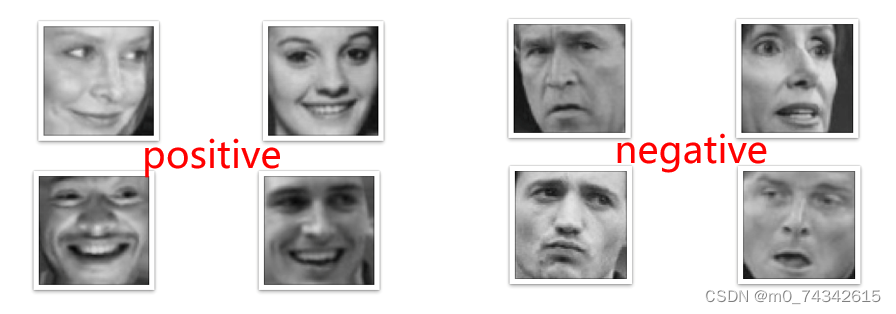
- 包含positive和negative两种表情,共7200余张图片
- 图片为16464,灰度图像
- 本次实验中,取其中的10%作为测试集,90%作为训练集
导入包
#倒入所需的包
import os
import zipfile
import random
import json
import cv2
import numpy as np
from PIL import Image
import paddle
import paddle.fluid as fluid
from multiprocessing import cpu_count
from paddle.fluid.dygraph import Linear
from paddle.fluid.dygraph import Pool2D,Conv2D
import matplotlib.pyplot as plt
配置参数
'''
参数配置
'''
train_parameters = {
    "input_size": [1, 32, 32],                           #输入图片的shape
    "class_dim": -1,                                     #分类数
    "src_path":"data/data33766/face_data.zip",          #原始数据集路径
    "target_path":"/home/aistudio/data/dataset",        #要解压的路径
    "train_list_path": "./train_data.txt",              #train_data.txt路径
    "eval_list_path": "./val_data.txt",                  #eval_data.txt路径
    "label_dict":{},                                    #标签字典
    "readme_path": "/home/aistudio/data/readme.json",   #readme.json路径
    "num_epochs": 2,                                    #训练轮数
    "train_batch_size": 8,                             #训练时每个批次的大小
    "learning_strategy": {                              #优化函数相关的配置
        "lr": 0.0001                                     #超参数学习率
    }
}
这段代码是对训练参数进行配置的。其中包括了输入图片的形状、分类数、原始数据集路径、要解压的路径、训练数据和评估数据的路径、标签字典、readme.json路径、训练轮数、训练时每个批次的大小以及优化函数相关的配置。其中学习率(lr)被设置为0.0001。这些参数将在训练模型时使用。
将原始数据集解压到指定目录下
def unzip_data(src_path,target_path):
    '''
    解压原始数据集,将src_path路径下的zip包解压至data/dataset目录下
    '''
    if(not os.path.isdir(target_path)):
        z = zipfile.ZipFile(src_path, 'r')
        z.extractall(path=target_path)
        z.close()
    else:
        print("文件已解压")
这段代码定义了一个名为unzip_data的函数,该函数接受两个参数src_path和target_path。函数的作用是解压原始数据集,将src_path路径下的zip包解压至data/dataset目录下。 在函数内部,首先通过os模块的isdir函数判断目标路径是否已存在,如果不存在,则使用zipfile模块的ZipFile函数打开src_path指定的zip包,然后调用extractall方法将其解压至target_path目录下,最后关闭zip文件。如果目标路径已存在,则打印"文件已解压"的提示信息。
生成数据列表
def get_data_list(target_path,train_list_path,eval_list_path):
    '''
    生成数据列表
    '''
    #存放所有类别的信息
    class_detail = []
    #获取所有类别保存的文件夹名称
    data_list_path=target_path
    class_dirs = os.listdir(data_list_path)
    if '__MACOSX'in class_dirs:
        class_dirs.remove('__MACOSX')
    if '.ipynb_checkpoints' in class_dirs:
        class_dirs.remove('.ipynb_checkpoints')
    # #总的图像数量
    all_class_images = 0
    # #存放类别标签
    class_label=0
    # #存放类别数目
    class_dim = 0
    # #存储要写进eval.txt和train.txt中的内容
    trainer_list=[]
    eval_list=[]
    # #读取每个类别,['positive', 'negative']
    for class_dir in class_dirs:
        if class_dir != ".DS_Store":
            class_dim += 1
            #每个类别的信息
            class_detail_list = {}
            eval_sum = 0
            trainer_sum = 0
            #统计每个类别有多少张图片
            class_sum = 0
            #获取类别路径
            path = os.path.join(data_list_path,class_dir)
            print(path)
            # 获取所有图片
            img_paths = os.listdir(path)
            for img_path in img_paths:                                  # 遍历文件夹下的每个图片
                if img_path =='.DS_Store':
                    continue
                name_path = os.path.join(path,img_path)                       # 每张图片的路径
                if class_sum % 10 == 0:                                 # 每10张图片取一个做验证数据
                    eval_sum += 1                                       # test_sum为测试数据的数目
                    eval_list.append(name_path + "\t%d" % class_label + "\n")
                else:
                    trainer_sum += 1
                    trainer_list.append(name_path + "\t%d" % class_label + "\n")#trainer_sum测试数据的数目
                class_sum += 1                                          #每类图片的数目
                all_class_images += 1                                   #所有类图片的数目

            # 说明的json文件的class_detail数据
            class_detail_list['class_name'] = class_dir             #类别名称
            class_detail_list['class_label'] = class_label          #类别标签
            class_detail_list['class_eval_images'] = eval_sum       #该类数据的测试集数目
            class_detail_list['class_trainer_images'] = trainer_sum #该类数据的训练集数目
            class_detail.append(class_detail_list)
            #初始化标签列表
            train_parameters['label_dict'][str(class_label)] = class_dir
            class_label += 1

    #初始化分类数
    train_parameters['class_dim'] = class_dim
    print(train_parameters)
    #乱序
    random.shuffle(eval_list)
    with open(eval_list_path, 'a') as f:
        for eval_image in eval_list:
            f.write(eval_image)

    random.shuffle(trainer_list)
    with open(train_list_path, 'a') as f2:
        for train_image in trainer_list:
            f2.write(train_image)

    # 说明的json文件信息
    readjson = {}
    readjson['all_class_name'] = data_list_path                  #文件父目录
    readjson['all_class_images'] = all_class_images
    readjson['class_detail'] = class_detail
    jsons = json.dumps(readjson, sort_keys=True, indent=4, separators=(',', ': '))
    with open(train_parameters['readme_path'],'w') as f:
        f.write(jsons)
    print ('生成数据列表完成!')
这段代码定义了一个名为get_data_list的函数,该函数接受三个参数target_path、train_list_path和eval_list_path。函数的作用是生成数据列表。在函数内部,首先定义了一个空列表class_detail来存放所有类别的信息。然后获取目标路径下的所有类别保存的文件夹名称,并排除一些特殊文件夹(如__MACOSX和.ipynb_checkpoints)。接着对每个类别进行遍历,统计每个类别有多少张图片,并将图片路径和类别标签写入到eval_list和trainer_list中。同时,也将每个类别的信息(类别名称、类别标签、测试集数目和训练集数目)存储到class_detail列表中。在遍历过程中,还初始化了标签列表和分类数目。最后,将eval_list和trainer_list乱序后写入到eval_list_path和train_list_path中,同时将数据信息存储到readme.json文件中。
自定义reader
def data_reader(file_list):
    '''
    自定义reader
    '''
    def reader():
        with open(file_list, 'r') as f:
            lines = [line.strip() for line in f]
            for line in lines:
                img_path, lab = line.strip().split('\t')
                img = Image.open(img_path)
                img = img.resize((32, 32), Image.ANTIALIAS)
                img = np.array(img).astype('float32')
                img = img/255.0
                yield img, int(lab)
    return reader
这段代码定义了一个名为data_reader的函数,该函数接受一个file_list参数,表示数据列表文件的路径。函数的作用是创建一个自定义的数据读取器。在函数内部,定义了一个名为reader的内部函数。reader函数使用了Python的生成器(generator)特性,它打开数据列表文件,逐行读取数据并进行预处理。首先,它读取每一行,并去除行末的换行符。然后,对每一行进行拆分,得到图片路径img_path和标签lab。接着,使用Pillow库(Python Imaging Library)的Image.open方法打开图片,并将其调整大小为32x32像素。然后将图像转换为NumPy数组,并将数据类型转换为float32。最后,将图像数据归一化到0到1之间,并使用yield语句产生一个(img, lab)的元组,其中img是处理后的图像数据,lab是对应的标签。
数据准备与数据提供器构造
'''
参数初始化
'''
src_path=train_parameters['src_path']
target_path=train_parameters['target_path']
train_list_path=train_parameters['train_list_path']
eval_list_path=train_parameters['eval_list_path']
batch_size=train_parameters['train_batch_size']
'''
解压原始数据到指定路径
'''
unzip_data(src_path,target_path)

'''
划分训练集与验证集,乱序,生成数据列表
'''
#每次生成数据列表前,首先清空train.txt和eval.txt
with open(train_list_path, 'w') as f:
    f.seek(0)
    f.truncate()
with open(eval_list_path, 'w') as f:
    f.seek(0)
    f.truncate()

#生成数据列表
get_data_list(target_path,train_list_path,eval_list_path)

'''
构造数据提供器
'''
train_reader = paddle.batch(data_reader(train_list_path),
                            batch_size=batch_size,
                            drop_last=True)
eval_reader = paddle.batch(data_reader(eval_list_path),
                            batch_size=batch_size,
                            drop_last=True)


/home/aistudio/data/dataset/Positive
/home/aistudio/data/dataset/Negative
{'input_size': [1, 32, 32], 'class_dim': 2, 'src_path': 'data/data33766/face_data.zip', 'target_path': '/home/aistudio/data/dataset', 'train_list_path': './train_data.txt', 'eval_list_path': './val_data.txt', 'label_dict': {'0': 'Positive', '1': 'Negative'}, 'readme_path': '/home/aistudio/data/readme.json', 'num_epochs': 2, 'train_batch_size': 8, 'learning_strategy': {'lr': 0.0001}}
生成数据列表完成!
这段代码是一个数据处理的流程,主要包括参数初始化、解压原始数据、划分训练集与验证集并生成数据列表、以及构造数据提供器。首先,通过train_parameters字典获取了一系列参数,包括原始数据路径(src_path)、目标数据路径(target_path)、训练集列表路径(train_list_path)、验证集列表路径(eval_list_path)和批处理大小(batch_size)等。接下来,调用unzip_data函数将原始数据解压到指定路径target_path。然后,清空并生成训练集和验证集的数据列表,通过调用get_data_list函数实现。在生成数据列表之后,会输出一个数据信息的json文件,标识生成数据列表的完成。最后,根据训练集和验证集的数据列表构造数据提供器train_reader和eval_reader,用于后续模型的训练和验证。
定义网络
#定义网络
class MyCNN(fluid.dygraph.Layer):
    def __init__(self):
        super(MyCNN,self).__init__()
        self.hidden1 = Conv2D(1,32,3,1)
        self.hidden2 = Conv2D(32,64,3,1)
        self.hidden3 = Pool2D(pool_size=2,pool_type='max',pool_stride=2)
        self.hidden4 = Conv2D(64,128,3,1)
        self.hidden5 = Linear(128*12*12,2,act='softmax')
    def forward(self,input):
        x = self.hidden1(input)
        # print(x.shape)
        x = self.hidden2(x)
        # print(x.shape)
        x = self.hidden3(x)
        # print(x.shape)
        x = self.hidden4(x)
        # print(x.shape)
        x = fluid.layers.reshape(x, shape=[-1, 128*12*12])
        y = self.hidden5(x)
        return y
这段代码定义了一个名为MyCNN的卷积神经网络模型,继承自fluid.dygraph.Layer类。在初始化方法__init__中,定义了神经网络的各个层,包括两个卷积层(hidden1和hidden2)、一个池化层(hidden3)、一个卷积层(hidden4)和一个全连接层(hidden5)。其中,卷积层使用了Conv2D类,池化层使用了Pool2D类,全连接层使用了Linear类。这些层的具体参数分别表示卷积核的数量、输入通道数、输出通道数、卷积核大小、步长、池化核大小、池化类型、池化步长等。在forward方法中,定义了数据在神经网络中的前向传播过程。输入数据input首先经过hidden1卷积层,然后经过hidden2卷积层,再经过hidden3池化层,接着经过hidden4卷积层,最后通过reshape将特征图展开成一维向量,然后输入到hidden5全连接层中,经过softmax激活函数得到最终的输出y。
绘制训练准确率和损失变化曲线
Batch=0
Batchs=[]
all_train_accs=[]
#定义draw_train_acc,绘制准确率变化曲线
def draw_train_acc(iters, train_accs):
    title="training accs"
    plt.title(title, fontsize=24)
    plt.xlabel("batch", fontsize=14)
    plt.ylabel("acc", fontsize=14)
    plt.plot(iters, train_accs, color='green', label='training accs')
    plt.legend()
    plt.grid()
    plt.show()
#定义draw_train_loss,绘制损失变化曲线
all_train_loss=[]
def draw_train_loss(iters, train_loss):
    title="training loss"
    plt.title(title, fontsize=24)
    plt.xlabel("batch", fontsize=14)
    plt.ylabel("loss", fontsize=14)
    plt.plot(iters, train_loss, color='red', label='training loss')
    plt.legend()
    plt.grid()
    plt.show()
这段代码定义了一些变量和函数,用于绘制训练过程中的准确率和损失变化曲线。首先,定义了变量Batch和Batchs,分别用于记录当前批次的训练数据数量和所有批次的训练数据数量。接着,定义了空列表all_train_accs和all_train_loss,用于存储所有批次的训练准确率和损失值。然后,定义了函数draw_train_acc和draw_train_loss,分别用于绘制训练准确率和损失的变化曲线。这两个函数接受两个参数iters和train_accs(或train_loss),分别表示迭代次数和对应的训练准确率(或损失)值。在函数内部,通过调用matplotlib库的绘图函数,将迭代次数和对应的准确率(或损失)值绘制成曲线图,并设置图表的标题、坐标轴标签、线条颜色等属性,最后通过plt.show()显示出图表。
使用动态图进行训练并绘制训练准确率和损失变化曲线
#用动态图进行训练
with fluid.dygraph.guard():
model = MyCNN()
model.train() #训练模式
opt=fluid.optimizer.AdamOptimizer(learning_rate=train_parameters['learning_strategy']['lr'], parameter_list=model.parameters())#优化器选用SGD随机梯度下降,学习率为0.001.
# epochs_num = train_parameters['num_epochs'] #迭代次数
epochs_num = 3 #迭代次数
for pass_num in range(epochs_num):
for batch_id,data in enumerate(train_reader()):
images=np.array([x[0].reshape(1,32,32) for x in data], np.float32)
labels = np.array([x[1] for x in data]).astype('int64')
labels = labels[:, np.newaxis]
image=fluid.dygraph.to_variable(images)
label=fluid.dygraph.to_variable(labels)
predict=model(image)
loss=fluid.layers.cross_entropy(predict,label)
avg_loss=fluid.layers.mean(loss)#获取loss值
acc=fluid.layers.accuracy(predict,label)#计算精度
if batch_id!=0 and batch_id%20==0:
Batch = Batch+20
Batchs.append(Batch)
all_train_loss.append(avg_loss.numpy()[0])
all_train_accs.append(acc.numpy()[0])
print("train_pass:{},batch_id:{},train_loss:{},train_acc:{}".format(pass_num,batch_id,avg_loss.numpy(),acc.numpy()))
avg_loss.backward()
opt.minimize(avg_loss)
model.clear_gradients()
fluid.save_dygraph(model.state_dict(),'MyCNN')#保存模型
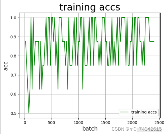
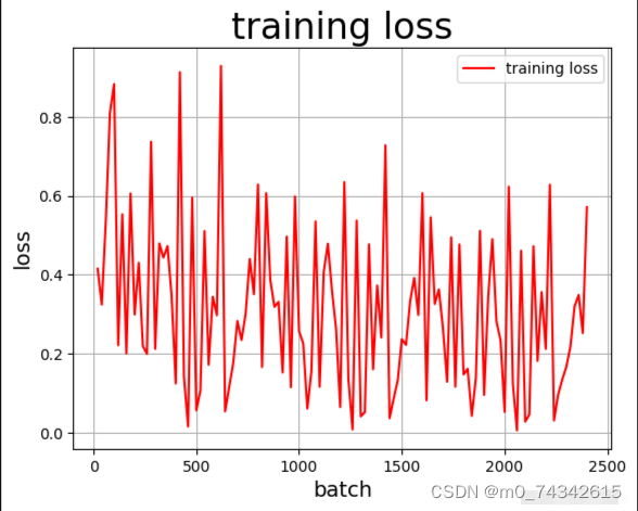
draw_train_acc(Batchs,all_train_accs)
draw_train_loss(Batchs,all_train_loss)运行结果如下
train_pass:0,batch_id:20,train_loss:[0.74191195],train_acc:[0.5]
train_pass:0,batch_id:40,train_loss:[0.7616366],train_acc:[0.5]
train_pass:0,batch_id:60,train_loss:[0.35878685],train_acc:[1.]
train_pass:0,batch_id:80,train_loss:[0.6831104],train_acc:[0.375]
train_pass:0,batch_id:100,train_loss:[0.24735436],train_acc:[1.]
train_pass:0,batch_id:120,train_loss:[0.3790019],train_acc:[0.875]
train_pass:0,batch_id:140,train_loss:[0.48425522],train_acc:[0.625]
train_pass:0,batch_id:160,train_loss:[0.91233456],train_acc:[0.625]
train_pass:0,batch_id:180,train_loss:[0.47714847],train_acc:[0.875]
train_pass:0,batch_id:200,train_loss:[0.15107517],train_acc:[1.]
train_pass:0,batch_id:220,train_loss:[0.63401103],train_acc:[0.625]
train_pass:0,batch_id:240,train_loss:[0.21741742],train_acc:[1.]
train_pass:0,batch_id:260,train_loss:[0.47167695],train_acc:[0.875]
train_pass:0,batch_id:280,train_loss:[0.34238392],train_acc:[0.75]
train_pass:0,batch_id:300,train_loss:[0.15976849],train_acc:[1.]
train_pass:0,batch_id:320,train_loss:[0.30184734],train_acc:[0.875]
train_pass:0,batch_id:340,train_loss:[0.3639618],train_acc:[0.875]
train_pass:0,batch_id:360,train_loss:[0.15780178],train_acc:[1.]
train_pass:0,batch_id:380,train_loss:[0.2903893],train_acc:[0.875]
train_pass:0,batch_id:400,train_loss:[0.19654405],train_acc:[0.875]
train_pass:0,batch_id:420,train_loss:[0.3627303],train_acc:[0.875]
train_pass:0,batch_id:440,train_loss:[0.24092944],train_acc:[1.]
train_pass:0,batch_id:460,train_loss:[0.6483213],train_acc:[0.75]
train_pass:0,batch_id:480,train_loss:[0.54234266],train_acc:[0.625]
train_pass:0,batch_id:500,train_loss:[0.5863033],train_acc:[0.5]
train_pass:0,batch_id:520,train_loss:[0.24061534],train_acc:[0.875]
train_pass:0,batch_id:540,train_loss:[0.24664079],train_acc:[1.]
train_pass:0,batch_id:560,train_loss:[0.08371078],train_acc:[1.]
train_pass:0,batch_id:580,train_loss:[0.45951968],train_acc:[0.875]
train_pass:0,batch_id:600,train_loss:[0.27173924],train_acc:[0.875]
train_pass:0,batch_id:620,train_loss:[0.29869416],train_acc:[1.]
train_pass:0,batch_id:640,train_loss:[0.06463003],train_acc:[1.]
train_pass:0,batch_id:660,train_loss:[0.7554905],train_acc:[0.875]
train_pass:0,batch_id:680,train_loss:[0.73131394],train_acc:[0.625]
train_pass:0,batch_id:700,train_loss:[0.16863066],train_acc:[0.875]
train_pass:0,batch_id:720,train_loss:[0.2530663],train_acc:[0.875]
train_pass:0,batch_id:740,train_loss:[0.53367794],train_acc:[0.875]
train_pass:0,batch_id:760,train_loss:[0.08805157],train_acc:[1.]
train_pass:0,batch_id:780,train_loss:[0.12519184],train_acc:[1.]
train_pass:0,batch_id:800,train_loss:[0.18847948],train_acc:[1.]
train_pass:1,batch_id:20,train_loss:[0.09347874],train_acc:[1.]
train_pass:1,batch_id:40,train_loss:[0.30578926],train_acc:[0.875]
train_pass:1,batch_id:60,train_loss:[0.11401831],train_acc:[1.]
train_pass:1,batch_id:80,train_loss:[0.45653576],train_acc:[0.75]
train_pass:1,batch_id:100,train_loss:[0.0845743],train_acc:[1.]
train_pass:1,batch_id:120,train_loss:[0.10384439],train_acc:[1.]
train_pass:1,batch_id:140,train_loss:[0.41081792],train_acc:[0.625]
train_pass:1,batch_id:160,train_loss:[0.34042948],train_acc:[0.875]
train_pass:1,batch_id:180,train_loss:[0.09779598],train_acc:[1.]
train_pass:1,batch_id:200,train_loss:[0.07199463],train_acc:[1.]
train_pass:1,batch_id:220,train_loss:[0.3792469],train_acc:[0.875]
train_pass:1,batch_id:240,train_loss:[0.21960266],train_acc:[0.875]
train_pass:1,batch_id:260,train_loss:[0.45843714],train_acc:[0.75]
train_pass:1,batch_id:280,train_loss:[0.21331987],train_acc:[0.875]
train_pass:1,batch_id:300,train_loss:[0.16417986],train_acc:[1.]
train_pass:1,batch_id:320,train_loss:[0.16865811],train_acc:[1.]
train_pass:1,batch_id:340,train_loss:[0.23856217],train_acc:[0.875]
train_pass:1,batch_id:360,train_loss:[0.22478923],train_acc:[0.875]
train_pass:1,batch_id:380,train_loss:[0.19512352],train_acc:[1.]
train_pass:1,batch_id:400,train_loss:[0.18784195],train_acc:[0.875]
train_pass:1,batch_id:420,train_loss:[0.4075334],train_acc:[0.75]
train_pass:1,batch_id:440,train_loss:[0.21361628],train_acc:[1.]
train_pass:1,batch_id:460,train_loss:[0.76711786],train_acc:[0.75]
train_pass:1,batch_id:480,train_loss:[0.45173714],train_acc:[0.875]
train_pass:1,batch_id:500,train_loss:[0.16800413],train_acc:[1.]
train_pass:1,batch_id:520,train_loss:[0.16689906],train_acc:[0.875]
train_pass:1,batch_id:540,train_loss:[0.36132887],train_acc:[0.75]
train_pass:1,batch_id:560,train_loss:[0.07532323],train_acc:[1.]
train_pass:1,batch_id:580,train_loss:[0.40087298],train_acc:[0.875]
train_pass:1,batch_id:600,train_loss:[0.2099344],train_acc:[1.]
train_pass:1,batch_id:620,train_loss:[0.1858334],train_acc:[1.]
train_pass:1,batch_id:640,train_loss:[0.04773728],train_acc:[1.]
train_pass:1,batch_id:660,train_loss:[0.71594566],train_acc:[0.875]
train_pass:1,batch_id:680,train_loss:[0.59711534],train_acc:[0.625]
train_pass:1,batch_id:700,train_loss:[0.17470069],train_acc:[0.875]
train_pass:1,batch_id:720,train_loss:[0.16642408],train_acc:[0.875]
train_pass:1,batch_id:740,train_loss:[0.5364364],train_acc:[0.875]
train_pass:1,batch_id:760,train_loss:[0.08197987],train_acc:[1.]
train_pass:1,batch_id:780,train_loss:[0.0879359],train_acc:[1.]
train_pass:1,batch_id:800,train_loss:[0.14894545],train_acc:[1.]
train_pass:2,batch_id:20,train_loss:[0.05806131],train_acc:[1.]
train_pass:2,batch_id:40,train_loss:[0.2726321],train_acc:[0.875]
train_pass:2,batch_id:60,train_loss:[0.08922889],train_acc:[1.]
train_pass:2,batch_id:80,train_loss:[0.36228722],train_acc:[0.75]
train_pass:2,batch_id:100,train_loss:[0.05018432],train_acc:[1.]
train_pass:2,batch_id:120,train_loss:[0.08069117],train_acc:[1.]
train_pass:2,batch_id:140,train_loss:[0.32687414],train_acc:[0.75]
train_pass:2,batch_id:160,train_loss:[0.32508028],train_acc:[0.875]
train_pass:2,batch_id:180,train_loss:[0.06988452],train_acc:[1.]
train_pass:2,batch_id:200,train_loss:[0.05463243],train_acc:[1.]
train_pass:2,batch_id:220,train_loss:[0.327322],train_acc:[0.875]
train_pass:2,batch_id:240,train_loss:[0.17910036],train_acc:[0.875]
train_pass:2,batch_id:260,train_loss:[0.40398407],train_acc:[0.75]
train_pass:2,batch_id:280,train_loss:[0.17278719],train_acc:[0.875]
train_pass:2,batch_id:300,train_loss:[0.15624687],train_acc:[1.]
train_pass:2,batch_id:320,train_loss:[0.15226051],train_acc:[1.]
train_pass:2,batch_id:340,train_loss:[0.18721214],train_acc:[0.875]
train_pass:2,batch_id:360,train_loss:[0.166887],train_acc:[1.]
train_pass:2,batch_id:380,train_loss:[0.18221357],train_acc:[1.]
train_pass:2,batch_id:400,train_loss:[0.19730295],train_acc:[0.875]
train_pass:2,batch_id:420,train_loss:[0.41209286],train_acc:[0.75]
train_pass:2,batch_id:440,train_loss:[0.20463249],train_acc:[0.875]
train_pass:2,batch_id:460,train_loss:[0.8085],train_acc:[0.75]
train_pass:2,batch_id:480,train_loss:[0.34228888],train_acc:[0.875]
train_pass:2,batch_id:500,train_loss:[0.12657],train_acc:[1.]
train_pass:2,batch_id:520,train_loss:[0.14959261],train_acc:[0.875]
train_pass:2,batch_id:540,train_loss:[0.37717828],train_acc:[0.75]
train_pass:2,batch_id:560,train_loss:[0.075846],train_acc:[1.]
train_pass:2,batch_id:580,train_loss:[0.35931224],train_acc:[0.875]
train_pass:2,batch_id:600,train_loss:[0.21139492],train_acc:[0.875]
train_pass:2,batch_id:620,train_loss:[0.17112082],train_acc:[1.]
train_pass:2,batch_id:640,train_loss:[0.05628181],train_acc:[1.]
train_pass:2,batch_id:660,train_loss:[0.64871454],train_acc:[0.875]
train_pass:2,batch_id:680,train_loss:[0.5126543],train_acc:[0.625]
train_pass:2,batch_id:700,train_loss:[0.18188927],train_acc:[0.875]
train_pass:2,batch_id:720,train_loss:[0.12543176],train_acc:[1.]
train_pass:2,batch_id:740,train_loss:[0.56217194],train_acc:[0.875]
train_pass:2,batch_id:760,train_loss:[0.0665126],train_acc:[1.]
train_pass:2,batch_id:780,train_loss:[0.06866351],train_acc:[1.]
train_pass:2,batch_id:800,train_loss:[0.12942857],train_acc:[1.]
<Figure size 432x288 with 1 Axes>
<Figure size 432x288 with 1 Axes>
模型评估
#模型评估
with fluid.dygraph.guard():
    accs = []
    model_dict, _ = fluid.load_dygraph('MyCNN')
    model = MyCNN()
    model.load_dict(model_dict) #加载模型参数
    model.eval() #训练模式
    for batch_id,data in enumerate(eval_reader()):#测试集
        images=np.array([x[0].reshape(1,32,32) for x in data],np.float32)
        labels = np.array([x[1] for x in data]).astype('int64')
        labels = labels[:, np.newaxis]
        image=fluid.dygraph.to_variable(images)
        label=fluid.dygraph.to_variable(labels)
        predict=model(image)
        acc=fluid.layers.accuracy(predict,label)
        accs.append(acc.numpy()[0])
        avg_acc = np.mean(accs)
    print(avg_acc)
0.8942308
综合来看,这段代码主要完成了加载模型参数、对测试集进行推理并计算准确率的过程,并输出了平均准确率。
使用预训练模型对图像进行预测评估
#读取预测图像,进行预处理
def load_image(path):
img = cv2.imread(path)
gray_image = cv2.cvtColor(img, cv2.COLOR_BGR2GRAY)
gray_image = cv2.resize(gray_image,(32,32))
gray_image = gray_image.reshape(1,32,32)
gray_image = np.array(gray_image).astype('float32')
gray_image = gray_image/255.0
return gray_image
infer_path = 'work/face_img.png'
#构建预测动态图过程
with fluid.dygraph.guard():
LABEL = train_parameters['label_dict']
print(train_parameters['label_dict'])
model=MyCNN()#模型实例化
model_dict,_=fluid.load_dygraph('MyCNN')
model.load_dict(model_dict)#加载模型参数
model.eval()#评估模式
infer_img = load_image(infer_path)
infer_img=np.array(infer_img).astype('float32')
infer_img=infer_img[np.newaxis, :]
print(infer_img.shape)
infer_img = fluid.dygraph.to_variable(infer_img)
result=model(infer_img)
print(result.numpy())
display(Image.open(infer_path))
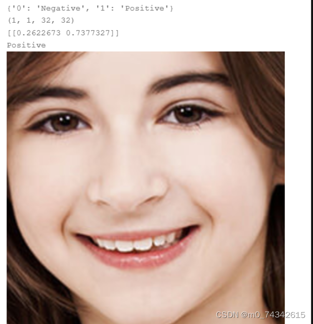
print(LABEL[str(np.argmax(result.numpy()))]){'0': 'Positive', '1': 'Negative'}
(1, 1, 32, 32)
[[0.64449733 0.35550264]]
Positive
<PIL.PngImagePlugin.PngImageFile image mode=RGBA size=440x440 at 0x7F207004CB50>