新闻分类（python深度学习——多分类问题）

记：新闻分类问题时多分类问题，与电影评论分类很类似又有一些差别，电影评论只有两个分类，而新闻分类有46个分类，所以在空间维度上有所增加，多分类问题的损失函数与二分类问题选择不同，最后一层使用的激活函数不同，其他基本流程都是一样的。

1、路透社数据集：包含许多短新闻及其对应的主题，是一个简单的，广泛使用的文本分类数据集，包含46个不同的主题，每个主题至少有10个样本，其中有8982个训练样本和2246个测试样本。

2、在编码标签时有两种方法（注意损失函数的选择是不同的）：

（1）将其转换为整数张量：

#转换为张量
y_train = np.array(train_labels)
y_test = np.array(test_labels)

#损失函数应选择：sparse_categorical_crossentropy
model.compile(optimezer='rmsprop',loss='sparse_categorical_crossentropy',metrics=['acc'])

(2)one-hot分类编码（两种实现方法）：

#①代码实现如下：

def to_one_hot(labels,dimension=46):
    results=np.zeros((len(labels),dimension))
    for i,label in enumerate(labels):
        results[i,label]=1.
    return results

#将训练标签和测试标签向量化
one_hot_train_labels=to_one_hot(train_labels)
one_hot_test_labels=to_one_hot(test_labels)

#②keras内置方法实现
one_hot_train_labels=to_categorical(train_labels)
one_hot_test_labels=to_categorical(test_labels)



#损失函数的选择为：categorical_crossentropy
model.compile(optimizer='rmsprop',
              loss='categorical_crossentropy',
              metrics=['accuracy'])

3、完整代码及部分注释如下：

#加载路透社数据集
from keras.datasets import reuters

(train_data,train_labels),(test_data,test_labels)=reuters.load_data(num_words=10000)

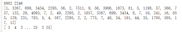
print(len(train_data),len(test_data))
print(train_data[1])
print(train_labels)

输出结果如下图：

#将索引解码为新闻文本(非必须，只是解码出来查看一下)
word_index=reuters.get_word_index()#将单词映射为整数索引的字典
reverse_word_index=dict([(value,key) for (key,value) in word_index.items()])#键值颠倒
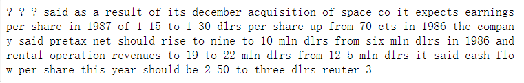
decoded_review=' '.join([reverse_word_index.get(i-3,'?') for i in train_data[0]])#解码，i-3是因为0，1，2是“填充”，“序列开始”，“未知词”


#查看解码后的数据
print(decoded_review)

解码后的新闻数据如下图：

#对数据进行编码
import numpy as np

#将整数序列编码为二进制矩阵，之后才能够将数据输入到神经网络中
def vectorize_sequences(sequences,dimension=10000):
    results=np.zeros((len(sequences),dimension))#创建一个该形状的零矩阵
    for i,sequence in enumerate(sequences):
        results[i,sequence]=1.
    return results

#将训练数据和测试数据向量化
x_train=vectorize_sequences(train_data)
x_test=vectorize_sequences(test_data)


#将标签进行向量化，有两种方法分别是：将标签列表转化为整数张量，或者使用one-hot分类编码，代码实现如下

def to_one_hot(labels,dimension=46):
    results=np.zeros((len(labels),dimension))
    for i,label in enumerate(labels):
        results[i,label]=1.
    return results

#将训练标签和测试标签向量化
one_hot_train_labels=to_one_hot(train_labels)
one_hot_test_labels=to_one_hot(test_labels)


#在keras内置方法可以实现这个操作，如下：
#one_hot_train_labels=to_categorical(train_labels)
#one_hot_test_labels=to_categorical(test_labels)


#构建网络，与电影评论分类不同的是，该问题的输出类别是46个，16维的空间无法区别46个分类，这个问题改成64维

#模型定义
from keras import models
from keras import layers

model=models.Sequential()
model.add(layers.Dense(64,activation='relu',input_shape=(10000,)))
model.add(layers.Dense(64,activation='relu'))
model.add(layers.Dense(46,activation='softmax'))


#编译模型
model.compile(optimizer='rmsprop',
              loss='categorical_crossentropy',
              metrics=['accuracy'])


#验证模型，留出1000个样本作为验证集
x_val=x_train[:1000]
partical_x_train=x_train[1000:]
y_val=one_hot_train_labels[:1000]
partical_y_train=one_hot_train_labels[1000:]


#训练模型，共20次迭代
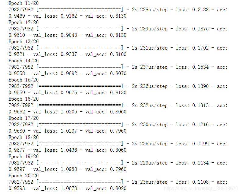
history=model.fit(partical_x_train,partical_y_train,
                  epochs=20,batch_size=512,
                  validation_data=(x_val,y_val))

迭代过程数据如下图所示：（非完整截图）

#绘制训练损失和验证损失图像

import matplotlib.pyplot as plt

history_dict=history.history
loss_values=history_dict['loss']
val_loss_values=history_dict['val_loss']

epochs=range(1,len(loss_values)+1)
plt.plot(epochs,loss_values,'bo',label='Training loss')#bo表示蓝色原点
plt.plot(epochs,val_loss_values,'b',label='Validation loss')#b表示蓝色实线
plt.title('training and validation loss')
plt.xlabel('Epochs')
plt.ylabel('Loss')
plt.legend()
plt.show()


#绘制训练精度和验证精度图像
#绘制训练和验证精度
plt.clf()   # clear figure
acc_values = history_dict['acc']
val_acc_values = history_dict['val_acc']

plt.plot(epochs, acc_values, 'bo', label='Training acc')
plt.plot(epochs, val_acc_values, 'b', label='Validation acc')
plt.title('Training and validation accuracy')
plt.xlabel('Epochs')
plt.ylabel('Accuracy')
plt.legend()

plt.show()

两幅图如下所示：

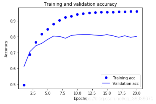
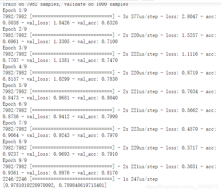
#如上图，在第9轮时出现了过拟合，现在我们重新训练一个网络，迭代9测，然后再测试集上进行评估
model = models.Sequential()
model.add(layers.Dense(64, activation='relu', input_shape=(10000,)))
model.add(layers.Dense(64, activation='relu'))
model.add(layers.Dense(46, activation='softmax'))
model.compile(optimizer='rmsprop',loss='categorical_crossentropy', metrics=['accuracy'])
model.fit(partical_x_train,partical_y_train,
          epochs=9,batch_size=512,
          validation_data=(x_val, y_val))
results = model.evaluate(x_test, one_hot_test_labels)

print(results)

测评结果如下图：（测试精度达到了78%）

#在新数据上生成预测结果

predict_result=model.predict(x_test)
print(predict_result.shape)
print(predict_result[0])
print(np.sum(predict_result[0]))

预测结果如下图所示：（因为使用的是softmax，所以最后所有预测结果的为1，或者逼近1）

新闻分类（python深度学习——多分类问题）

悦读