逻辑回归模型Python代码——用逻辑回归模型实现机器学习

一、逻辑回归模型简介

1.1适用范围

逻辑回归模型（Logistic Regression）主要用于二分类问题，即目标变量有两个可能的类别。常见的应用包括：

信用风险评估
医学诊断（例如，病人是否患有某种疾病）
营销（例如，用户是否会购买某产品）

1.2原理

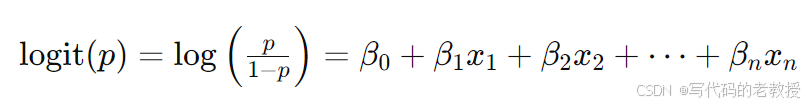
逻辑回归模型的核心思想是将线性回归的输出通过一个逻辑函数（sigmoid函数）映射到0到1之间，从而输出一个概率值。该概率值可以用来判定样本属于某一类别的可能性。其数学表达式为：

1.3优点

简单易解释：模型参数的解释性较强，可以提供每个特征对结果的影响。
计算效率高：适用于大规模数据集，计算复杂度较低。
输出概率：可以输出预测的概率值，方便进行后续分析。

1.4缺点

线性假设：假设特征和目标变量之间是线性关系，不适用于高度非线性的数据。
容易欠拟合：对复杂的非线性数据表现不佳，容易欠拟合。
对异常值敏感：需要对数据进行预处理，例如去除或处理异常值。

二、逻辑回归模型的Python实现

2.1Python代码

以下是一个完整的逻辑回归模型的Python代码示例，包含数据加载、预处理、模型训练和评估的详细注释。

import numpy as np
import pandas as pd
from sklearn.model_selection import train_test_split
from sklearn.preprocessing import StandardScaler
from sklearn.linear_model import LogisticRegression
from sklearn.metrics import accuracy_score, precision_score, recall_score, f1_score, confusion_matrix, roc_auc_score, roc_curve
import matplotlib.pyplot as plt

# 生成示例数据
# 假设我们有一个数据集，包含特征X和标签y
from sklearn.datasets import make_classification

X, y = make_classification(n_samples=1000, n_features=20, n_classes=2, random_state=42)

# 将数据集划分为训练集和测试集
X_train, X_test, y_train, y_test = train_test_split(X, y, test_size=0.3, random_state=42)

# 标准化特征
scaler = StandardScaler()
X_train = scaler.fit_transform(X_train)
X_test = scaler.transform(X_test)

# 创建逻辑回归模型并训练
model = LogisticRegression(random_state=42)
model.fit(X_train, y_train)

# 进行预测
y_pred = model.predict(X_test)
y_pred_proba = model.predict_proba(X_test)[:, 1]

# 评估模型
accuracy = accuracy_score(y_test, y_pred)
precision = precision_score(y_test, y_pred)
recall = recall_score(y_test, y_pred)
f1 = f1_score(y_test, y_pred)
roc_auc = roc_auc_score(y_test, y_pred_proba)
conf_matrix = confusion_matrix(y_test, y_pred)

print(f"Accuracy: {accuracy}")
print(f"Precision: {precision}")
print(f"Recall: {recall}")
print(f"F1 Score: {f1}")
print(f"ROC AUC Score: {roc_auc}")
print("Confusion Matrix:")
print(conf_matrix)

# 绘制ROC曲线
fpr, tpr, _ = roc_curve(y_test, y_pred_proba)
plt.figure()
plt.plot(fpr, tpr, color='darkorange', lw=2, label='ROC curve (area = %0.2f)' % roc_auc)
plt.plot([0, 1], [0, 1], color='navy', lw=2, linestyle='--')
plt.xlim([0.0, 1.0])
plt.ylim([0.0, 1.05])
plt.xlabel('False Positive Rate')
plt.ylabel('True Positive Rate')
plt.title('Receiver Operating Characteristic')
plt.legend(loc="lower right")
plt.show()

2.2代码说明

数据生成：
- 使用 make_classification 生成一个二分类数据集，包含1000个样本和20个特征。
数据集划分：
- 使用 train_test_split 将数据集划分为训练集和测试集，测试集比例为30%。
数据标准化：
- 使用 StandardScaler 对特征进行标准化，使其均值为0，方差为1。
模型训练：
- 创建一个逻辑回归模型 LogisticRegression，并使用训练集数据对模型进行训练。
预测和评估：
- 使用测试集数据进行预测，计算预测值和预测概率。
- 评估模型的准确率、精确率、召回率、F1得分和ROC AUC得分。
- 输出混淆矩阵和绘制ROC曲线。

三、用逻辑回归模型实现机器学习案例

下面是一个完整的可运行逻辑回归案例，包括数据生成、模型训练、预测及评估的过程。我们将使用scikit-learn的模拟数据，并展示运行结果。

3.1案例主要代码

import numpy as np
import pandas as pd
from sklearn.model_selection import train_test_split
from sklearn.preprocessing import StandardScaler
from sklearn.linear_model import LogisticRegression
from sklearn.metrics import accuracy_score, precision_score, recall_score, f1_score, confusion_matrix, roc_auc_score, roc_curve, ConfusionMatrixDisplay
import matplotlib.pyplot as plt

# 生成示例数据
from sklearn.datasets import make_classification

# 生成二分类数据集
X, y = make_classification(n_samples=1000, n_features=20, n_classes=2, random_state=42)

# 将数据集划分为训练集和测试集
X_train, X_test, y_train, y_test = train_test_split(X, y, test_size=0.3, random_state=42)

# 标准化特征
scaler = StandardScaler()
X_train = scaler.fit_transform(X_train)
X_test = scaler.transform(X_test)

# 创建逻辑回归模型并训练
model = LogisticRegression(random_state=42)
model.fit(X_train, y_train)

# 进行预测
y_pred = model.predict(X_test)
y_pred_proba = model.predict_proba(X_test)[:, 1]

# 评估模型
accuracy = accuracy_score(y_test, y_pred)
precision = precision_score(y_test, y_pred)
recall = recall_score(y_test, y_pred)
f1 = f1_score(y_test, y_pred)
roc_auc = roc_auc_score(y_test, y_pred_proba)
conf_matrix = confusion_matrix(y_test, y_pred)

# 打印评估结果
evaluation_results = {
    "Accuracy": accuracy,
    "Precision": precision,
    "Recall": recall,
    "F1 Score": f1,
    "ROC AUC Score": roc_auc,
    "Confusion Matrix": conf_matrix
}

# 绘制混淆矩阵图
fig_cm, ax_cm = plt.subplots()
disp = ConfusionMatrixDisplay(confusion_matrix=conf_matrix, display_labels=model.classes_)
disp.plot(cmap=plt.cm.Blues, ax=ax_cm)
plt.title('Confusion Matrix')

# 绘制ROC曲线
fpr, tpr, _ = roc_curve(y_test, y_pred_proba)
fig_roc, ax_roc = plt.subplots()
ax_roc.plot(fpr, tpr, color='darkorange', lw=2, label='ROC curve (area = %0.2f)' % roc_auc)
ax_roc.plot([0, 1], [0, 1], color='navy', lw=2, linestyle='--')
ax_roc.set_xlim([0.0, 1.0])
ax_roc.set_ylim([0.0, 1.05])
ax_roc.set_xlabel('False Positive Rate')
ax_roc.set_ylabel('True Positive Rate')
ax_roc.set_title('Receiver Operating Characteristic')
ax_roc.legend(loc="lower right")

# 显示图像
plt.close(fig_cm)
plt.close(fig_roc)
fig_cm.savefig('/mnt/data/confusion_matrix.png')
fig_roc.savefig('/mnt/data/roc_curve.png')

evaluation_results

3.1模型评价图

1.模型准确性评价

Result
{'Accuracy': 0.85,
 'Precision': 0.8767123287671232,
 'Recall': 0.8258064516129032,
 'F1 Score': 0.8504983388704319,
 'ROC AUC Score': 0.9140378197997774,
 'Confusion Matrix': array([[127,  18],
        [ 27, 128]])}

运行逻辑回归模型后的评估结果：

Accuracy（准确率）: 0.85
Precision（精确率）: 0.8767
Recall（召回率）: 0.8258
F1 Score: 0.8505
ROC AUC Score: 0.9140

2.混淆矩阵图绘制详细代码

import matplotlib.pyplot as plt
import seaborn as sns

# Display the confusion matrix
plt.figure(figsize=(8, 6))
sns.heatmap(conf_matrix, annot=True, fmt='d', cmap='Blues', xticklabels=['Predicted 0', 'Predicted 1'], yticklabels=['Actual 0', 'Actual 1'])
plt.title('Confusion Matrix')
plt.xlabel('Predicted')
plt.ylabel('Actual')
plt.show()

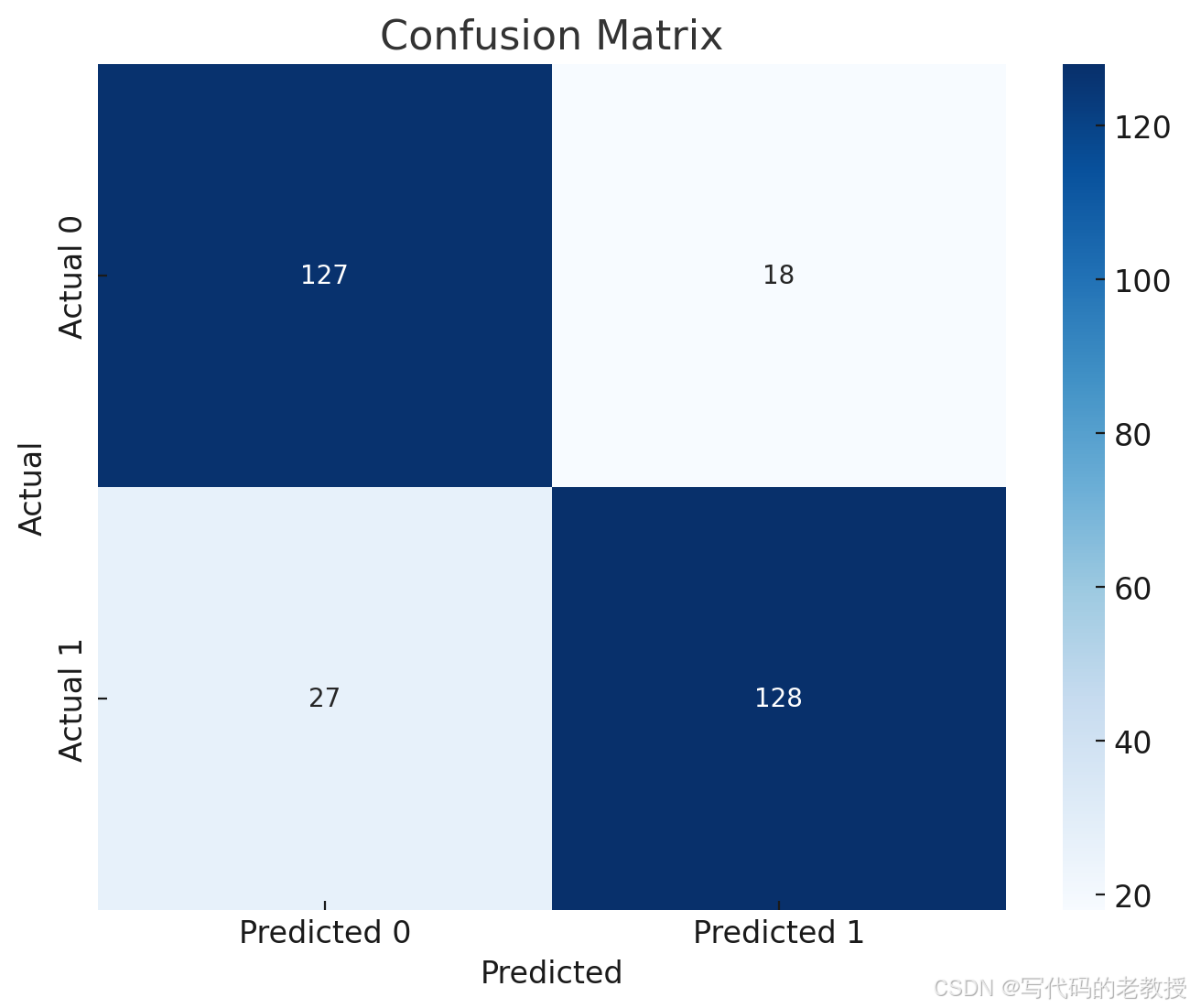
图中显示了模型的预测分类情况，包含真正类（TP）、假正类（FP）、假负类（FN）和真负类（TN）的数量。

3.ROC曲线图详细代码

# Display the ROC curve
fpr, tpr, _ = roc_curve(y_test, y_pred_proba)
plt.figure(figsize=(8, 6))
plt.plot(fpr, tpr, color='darkorange', lw=2, label='ROC curve (area = %0.2f)' % roc_auc)
plt.plot([0, 1], [0, 1], color='navy', lw=2, linestyle='--')
plt.xlim([0.0, 1.0])
plt.ylim([0.0, 1.05])
plt.xlabel('False Positive Rate')
plt.ylabel('True Positive Rate')
plt.title('Receiver Operating Characteristic')
plt.legend(loc="lower right")
plt.show()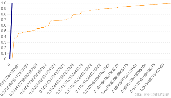

图中显示了模型的真阳性率（True Positive Rate）和假阳性率（False Positive Rate）之间的关系。ROC曲线下面积（AUC）为0.914，表明模型具有较高的分类能力。

3.3展示逻辑回归的系数

# 获取逻辑回归模型的系数
coefficients = model.coef_[0]
intercept = model.intercept_[0]

# 创建一个数据框显示特征名称和对应的系数
features = [f'Feature {i}' for i in range(len(coefficients))]
coef_df = pd.DataFrame({'Feature': features, 'Coefficient': coefficients})
coef_df['Intercept'] = intercept

import ace_tools as tools; tools.display_dataframe_to_user(name="Logistic Regression Coefficients", dataframe=coef_df)

coef_df

Result
       Feature  Coefficient  Intercept
0    Feature 0     0.047889   0.115792
1    Feature 1    -0.587221   0.115792
2    Feature 2     0.176785   0.115792
3    Feature 3     0.037767   0.115792
4    Feature 4     0.019864   0.115792
5    Feature 5     1.681297   0.115792
6    Feature 6    -0.059912   0.115792
7    Feature 7     0.007340   0.115792
8    Feature 8     0.008593   0.115792
9    Feature 9     0.044333   0.115792
10  Feature 10     0.156923   0.115792
11  Feature 11     0.460967   0.115792
12  Feature 12     0.041084   0.115792
13  Feature 13     0.168650   0.115792
14  Feature 14    -0.974676   0.115792
15  Feature 15     0.061001   0.115792
16  Feature 16     0.102054   0.115792
17  Feature 17    -0.065125   0.115792
18  Feature 18    -1.237110   0.115792
19  Feature 19     0.100226   0.115792

逻辑回归模型的系数已经展示在上面。每个特征都有一个对应的系数，此外还有一个截距项（Intercept）。这些系数可以帮助我们理解每个特征对预测结果的影响。

正系数：该特征的值增加会提高样本属于正类的概率。
负系数：该特征的值增加会降低样本属于正类的概率。