这篇文章是对前段时间机器学习内容的总结和回顾，能为继续学习者，做个指引；十分感谢协会的组织，老师的讲解，还有在一起辛苦学习的小伙伴们。勤奋耕耘，付出总有收获。大家在阅读的过程中，有什么问题，或者改进的建议，或者书写错误的地方，请指出，方便大家更好的阅读。谢谢大家的支持！

1 环境配置

1.1 Python

python的安装包：python 3.8

1.2 配置anaconda

参考地址：https://mirrors.tuna.tsinghua.edu.cn/anaconda/archive/

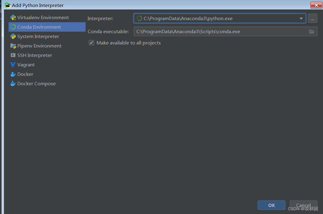
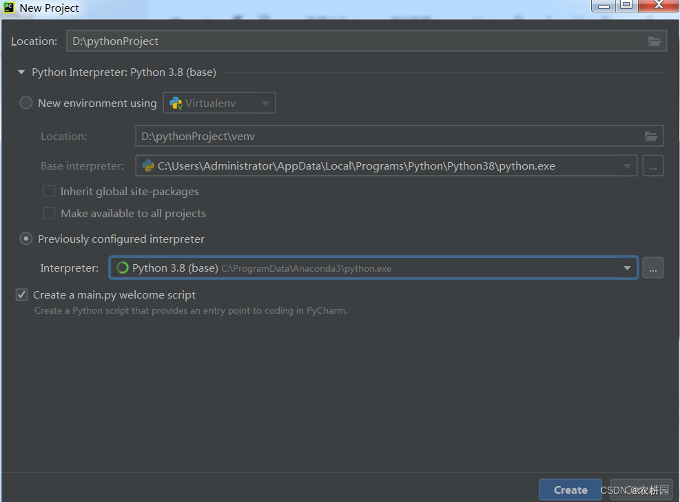
1.3 安装pycharm

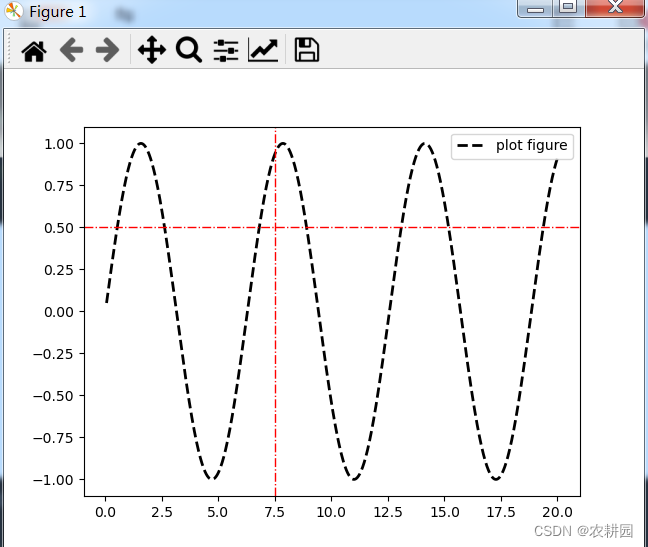
1.4 绘制plot figure

import matplotlib.pyplot as plt
import numpy as np
x = np.linspace(0.05,20,2000)
y = np.sin(x)
plt.plot(x,y,ls='--',c='k',lw=2,label='plot figure')
plt.legend()
plt.axhline(0.5,ls='-.',c='r',lw=1)
plt.axvline(7.5,ls='-.',c='r',lw=1)
plt.savefig('E:\\test\\test.png',dpi=300)
plt.show()

结果：

2 数据分析

2.1 预测房价

第一种方式：

def cal_price(city, area):
    if area<0:
        print('面积输入错误，请重新输入！')
        return 0
    if city == "深圳":
        if area < 100:
            return area * 70000
        else:
            return area * 60000
    elif city == "广州":
        if area < 90:
            return area * 40000
        else:
            return area * 30000
    else:
        return area * 60000
print("请输入城市名称：")
city = input()
print("请输入房屋面积：")
area = int(input())
house_price = cal_price(city, area)
if house_price==0:
    print('输入错误，请重新输入！')
else:
    print("房屋的价格：%d" % house_price)

结果：

C:\ProgramData\Anaconda3\python.exe D:/test/test.py
请输入城市名称：
深圳
请输入房屋面积：
300
房屋的价格：18000000

进程已结束，退出代码为 0

第二种方式：

def cal_price(city,squar):
    if squar <0:
        print('面积输入错误，请重新输入！')
        return 0
    if  city == "深圳":
        if squar < 100:
           HP = squar * 7
        else:
            HP = squar * 6
    elif city =="广州":
        if squar < 90:
           HP = squar * 4
        else:
            HP = squar * 3
    else:
        HP =squar * 6
    return HP

def main():
    city = input("请输入你的城市：")
    squar = int(input("请输入房子的面积："))
    price= cal_price(city,squar)
    print("您的房价是:" + str(price))

if __name__ == '__main__':
    main()

第三种方式：

def GetHousePrice(city,area):
    if city =='深圳':
        if area < 100:
            HP = 7 * area
        else:
            HP = 6 * area
    elif city == '广州':
        if area < 90:
            HP = 4 * area
        else:
            HP = 3 * area
    else:
        HP = 6 * area
    return HP

def main():
    city = input("请输入你的城市：")
    area = int(input("请输入房子的面积："))
    HP = GetHousePrice(city,area)
    print("您的房价是:"+str(HP))

if __name__ == '__main__':
    main()

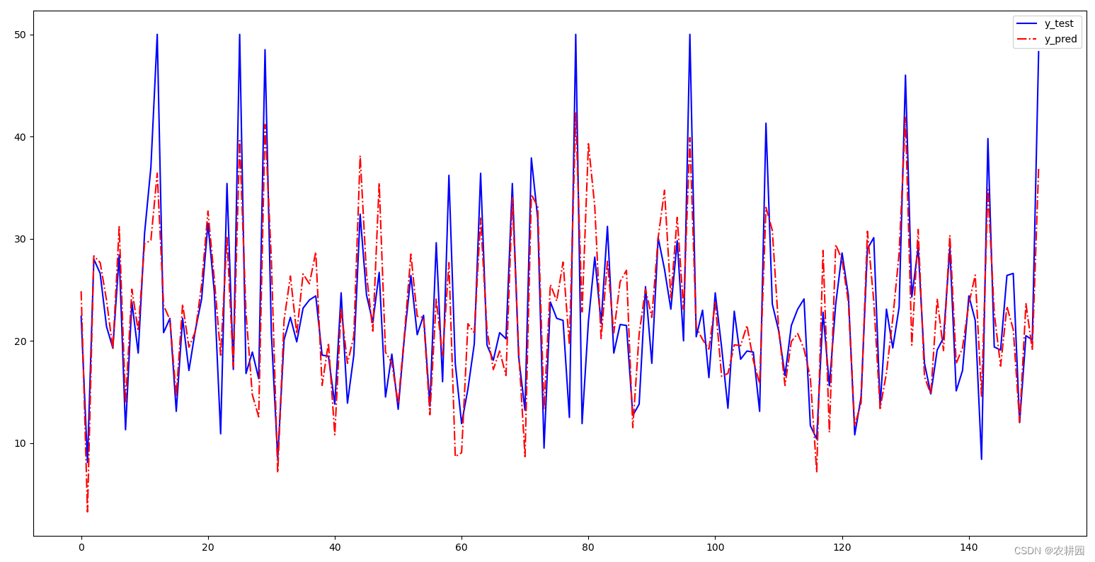
2.2 预测波士顿房价

from sklearn.linear_model import LinearRegression #导入线性回归
from sklearn.datasets import load_boston #导入波士顿的数据集
from sklearn.model_selection import train_test_split #模型划分，训练集，测试集

boston = load_boston()
print(boston)

x = boston['data']  #取出boston字典里的data数据
y = boston['target'] #取出boston字典里边的target数据

#1、划分训练集和测试集  特征数据x  标签数据y  训练集 x_train y_train 测试集 x_test y_test
from sklearn.model_selection import train_test_split
x_train,x_test,y_train,y_test = train_test_split(x,y,test_size=0.3)

#2和3
model_test =LinearRegression().fit(x_train,y_train)
#4、预测
y_pred = model_test.predict(x_test)
print(y_pred)

#图形展示
import matplotlib.pyplot as plt
plt.plot(range(y_test.shape[0]),y_test,color='blue',linewidth=1.5,linestyle='-')
plt.plot(range(y_test.shape[0]),y_pred,color='red',linewidth=1.5,linestyle='-.')
plt.legend(['y_test','y_pred'])
plt.show()

结果：

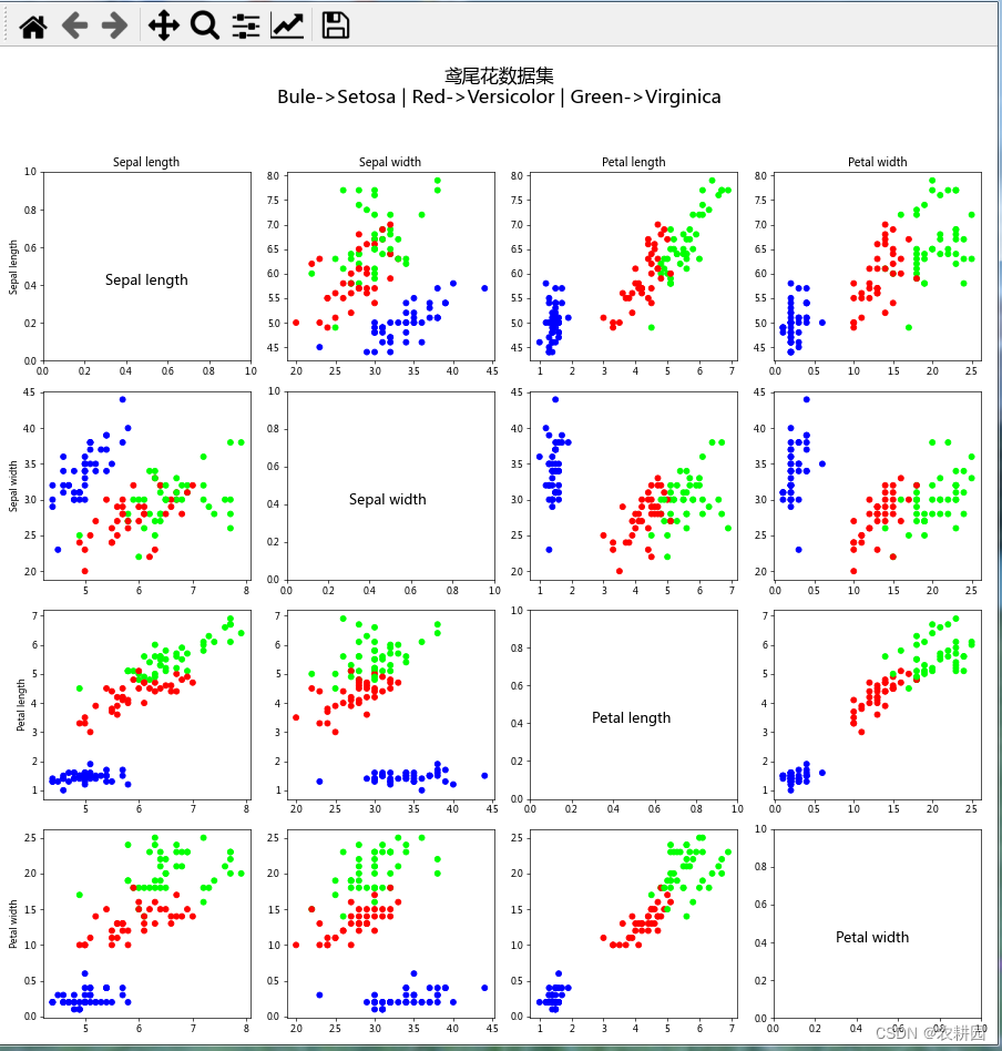
2.3 鸢尾花的算法

第一种方式：

import matplotlib.pyplot as plt
import numpy as np
import tensorflow as tf
import pandas as pd
plt.rcParams['font.sans-serif'] = ['Microsoft YaHei']
plt.rcParams['axes.unicode_minus'] = False
TRAIN_URL = r'http://download.tensorflow.org/data/iris_training.csv'
train_path = tf.keras.utils.get_file(TRAIN_URL.split('/')[-1], TRAIN_URL)
names = ['Sepal length', 'Sepal width', 'Petal length', 'Petal width', 'Species']
df_iris = pd.read_csv(train_path, header=0, names=names)
iris_data = df_iris.values
plt.figure(figsize=(15, 15), dpi=60)
for i in range(4):
    for j in range(4):
        plt.subplot(4, 4, i * 4 + j + 1)
        if i == 0:
            plt.title(names[j])
        if j == 0:
            plt.ylabel(names[i])
        if i == j:
            plt.text(0.3, 0.4, names[i], fontsize=15)
            continue
        plt.scatter(iris_data[:, j], iris_data[:, i], c=iris_data[:, -1], cmap='brg')
plt.tight_layout(rect=[0, 0, 1, 0.9])
plt.suptitle('鸢尾花数据集\nBule->Setosa | Red->Versicolor | Green->Virginica', fontsize=20)
plt.show()

结果：

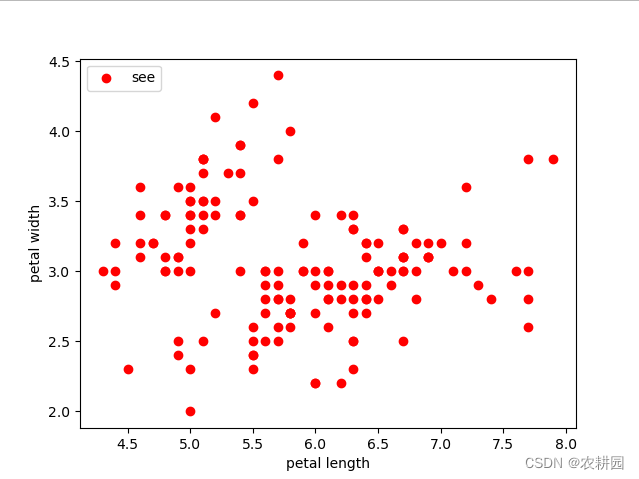
第二种方式：

from sklearn import datasets
from sklearn.cluster import KMeans
import matplotlib.pyplot as plt

iris = datasets.load_iris()
# 2.取特征空间中的4个维度
X = iris.data[:, :4]
# 3.搭建模型，构造KMeans聚类器，聚类个数为3
estimator = KMeans(n_clusters=3)
#开始聚类训练
estimator.fit(X)
# 获取聚类标签
label_pred = estimator.labels_
# 绘制数据分布图（数据可视化）
plt.scatter(X[:, 0], X[:, 1], c="red", marker='o', label='see')
plt.xlabel('petal length')
plt.ylabel('petal width')
plt.legend(loc=2)
plt.show()
# 绘制k-means结果
x0 = X[label_pred == 0]
x1 = X[label_pred == 1]
x2 = X[label_pred == 2]
plt.scatter(x0[:, 0], x0[:, 1], c="red", marker='o', label='label0')
plt.scatter(x1[:, 0], x1[:, 1], c="green", marker='*', label='label1')
plt.scatter(x2[:, 0], x2[:, 1], c="blue", marker='+', label='label2')
#花瓣的长宽
plt.xlabel('petal length')
plt.ylabel('petal width')
plt.legend(loc=2)
plt.show()

结果：

第三种方式：

from sklearn.datasets import load_iris
from sklearn.model_selection import train_test_split
from sklearn.neighbors import KNeighborsClassifier
import numpy as np
# 载入数据集
iris_dataset = load_iris()
# 数据划分
X_train, X_test, y_train, y_test = train_test_split(iris_dataset['data'], iris_dataset['target'], random_state=0)
# 设置邻居数
knn = KNeighborsClassifier(n_neighbors=1)
# 构建基于训练集的模型
knn.fit(X_train, y_train)
# 一条测试数据
X_new = np.array([[5, 2.9, 1, 0.2]])
# 对X_new预测结果
prediction = knn.predict(X_new)
print("预测值%d" % prediction)
# 得出测试集X_test测试集的分数
print("score:{:.2f}".format(knn.score(X_test, y_test)))

结果：

2.4 根据Excel中每列进行展示

import pandas as pd
import numpy as np
import matplotlib.pyplot as plt
plt.rcParams["font.sans-serif"] =["SimHei"] #设置字体
plt.rcParams["axes.unicode_minus"] =False #该语句解决图像种的“-”负号的乱码问题

#读取原始文件内容
ori_data = pd.read_excel(r"E:\test\客户数据-all-1.xlsx")
#初步筛选出已经购买课程的群体
df = pd.DataFrame(ori_data[ori_data["是否购买课程"]==1])
#先获取表格中的列名
columns_name = np.array(df.columns)
#输入列名
print(columns_name)

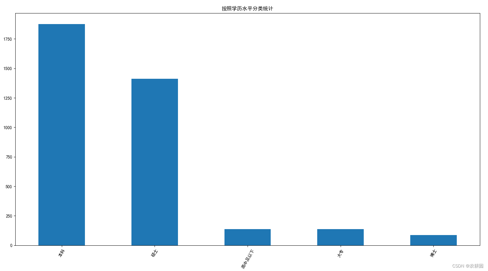
def statistics_classification(name):
    #筛选出需要的数据并且回执条形图形
    df[name].value_counts().plot(kind="bar")
    #图形标题
    plt.title("按照"+name+"分类统计")
    #X坐标轴显示旋转
    plt.xticks(rotation=60)
    plt.show()

name = input("请输入想要筛选的内容:")
if name not in columns_name:
    print("输入的内容错误")
else:
    statistics_classification(name)

结果：

C:\ProgramData\Anaconda3\python.exe D:/test/test.py
['Unnamed: 0' 'Unnamed: 0.1' 'Unnamed: 0.1.1' '手机号' '性别' '年龄' '学历水平'
 '婚姻状态' '常居城市' '子女年龄' '是否购买过少儿课程' '是否体验过本课程' '是否购买过少儿保险' '客户财富等级'
 '是否去过高端商场' '是否去过高尔夫球场' '是否住在高端小区' '是否喜欢旅游' '是否出过国' '客户是否有房' '房价' '是否有车'
 '销售渠道' '行业分类' '英语水平' '健康状况' '是否购买课程']
请输入想要筛选的内容:学历水平

3 神经网络

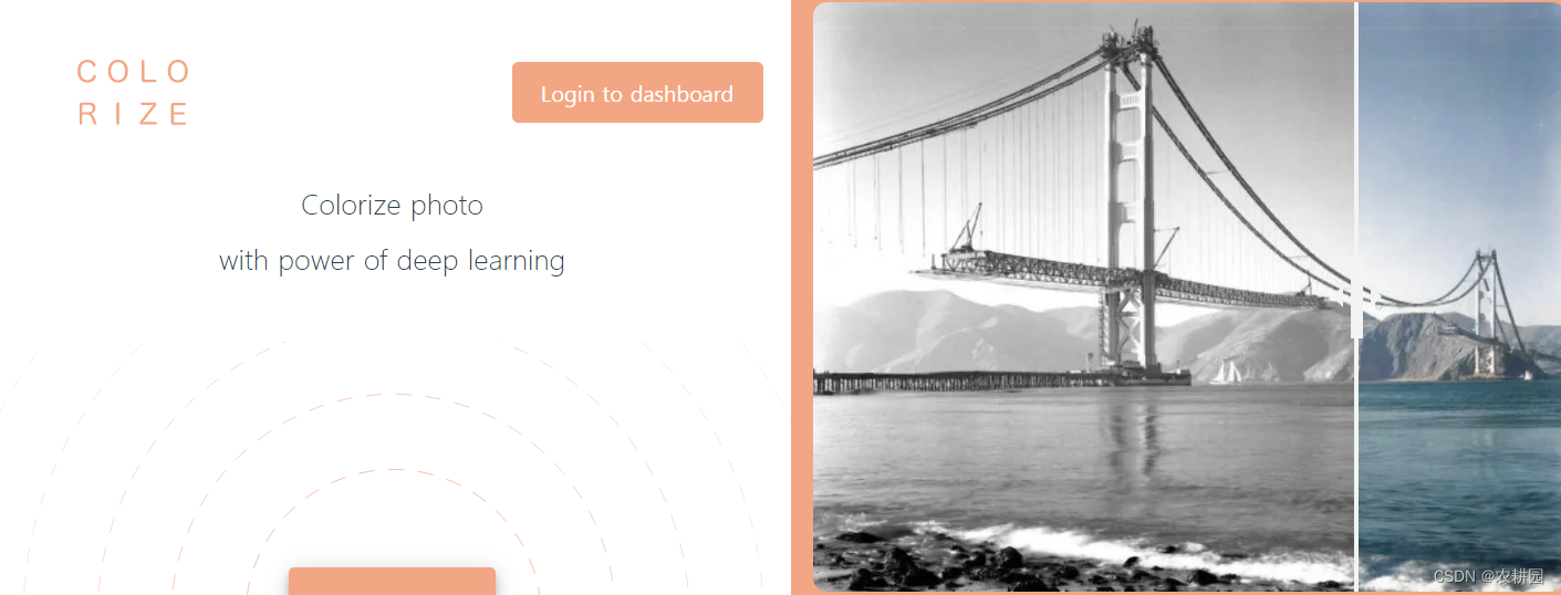
3.1 图片处理工具

https://colorize.cc/

https://cloud.baidu.com/product/imageprocess/colourize?track=cp:nsem%7Cpf:PC%7Cpp:P-fengchao124-tuxiangzengqiangtexiao-bayue%7Cpu:heibaitupianshangse%7Cci:%7Ckw:10368400&bd_vid=9996180438037139433

3.2 安装tensorflow

pip install -i https://pypi.tuna.tsinghua.edu.cn/simple tensorflow==2.6.0

3.3 预测房价

dict = {'深圳':80,'广州':90}
print(dict)
city=input("请输入城市：")
# area=input("请输入面积：")
for d in dict:
    if d == city and city == '深圳':
        print(d)
        price = dict[d] * 7
        break;
    elif d == city and city == '广州':
        print(d)
        price = dict[d] * 6
        break;
print(price)

结果：

C:\ProgramData\Anaconda3\python.exe D:/test/test.py
{'深圳': 80, '广州': 90}
请输入城市：广州
广州
540

3.4 生成矩阵

![# import tensorflow as tf
# tf.__version__
# print(tf.__version__)
# # 常量
# a =tf.constant(3)
# b =tf.constant(2)
#
# #生成一个1*3的数组
# c =tf.Variable(tf.constant([1,2,3]))
# print(c)在这里插入图片描述


#
# #生成矩阵
# c0= tf.zeros([10,33])
# c1= tf.ones([10,33])
# c2= tf.fill([10,33],2.)
#
# #矩阵的运算
# print('c2+c1',tf.add(c2,c1))
# print('c2-c1',tf.subtract(c1,c2))
# #乘法
# print('c2+c1',tf.multiply(c2,c1))
# #除法
# print('c2+c1',tf.divide(c2,c1))
# print(c1)]

结果：

C:\ProgramData\Anaconda3\python.exe D:/test/test.py
2022-07-12 16:19:55.812000: W tensorflow/stream_executor/platform/default/dso_loader.cc:64] Could not load dynamic library 'cudart64_110.dll'; dlerror: cudart64_110.dll not found
2022-07-12 16:19:55.869000: I tensorflow/stream_executor/cuda/cudart_stub.cc:29] Ignore above cudart dlerror if you do not have a GPU set up on your machine.
2.6.0
2022-07-12 16:20:56.844000: W tensorflow/stream_executor/platform/default/dso_loader.cc:64] Could not load dynamic library 'cudart64_110.dll'; dlerror: cudart64_110.dll not found
2022-07-12 16:20:56.846000: W tensorflow/stream_executor/platform/default/dso_loader.cc:64] Could not load dynamic library 'cublas64_11.dll'; dlerror: cublas64_11.dll not found
2022-07-12 16:20:56.849000: W tensorflow/stream_executor/platform/default/dso_loader.cc:64] Could not load dynamic library 'cublasLt64_11.dll'; dlerror: cublasLt64_11.dll not found
2022-07-12 16:20:56.851000: W tensorflow/stream_executor/platform/default/dso_loader.cc:64] Could not load dynamic library 'cufft64_10.dll'; dlerror: cufft64_10.dll not found
2022-07-12 16:20:56.855000: W tensorflow/stream_executor/platform/default/dso_loader.cc:64] Could not load dynamic library 'curand64_10.dll'; dlerror: curand64_10.dll not found
2022-07-12 16:20:56.857000: W tensorflow/stream_executor/platform/default/dso_loader.cc:64] Could not load dynamic library 'cusolver64_11.dll'; dlerror: cusolver64_11.dll not found
2022-07-12 16:20:56.860000: W tensorflow/stream_executor/platform/default/dso_loader.cc:64] Could not load dynamic library 'cusparse64_11.dll'; dlerror: cusparse64_11.dll not found
2022-07-12 16:20:56.863000: W tensorflow/stream_executor/platform/default/dso_loader.cc:64] Could not load dynamic library 'cudnn64_8.dll'; dlerror: cudnn64_8.dll not found
2022-07-12 16:20:56.863000: W tensorflow/core/common_runtime/gpu/gpu_device.cc:1835] Cannot dlopen some GPU libraries. Please make sure the missing libraries mentioned above are installed properly if you would like to use GPU. Follow the guide at https://www.tensorflow.org/install/gpu for how to download and setup the required libraries for your platform.
Skipping registering GPU devices...
2022-07-12 16:20:56.938000: I tensorflow/core/platform/cpu_feature_guard.cc:142] This TensorFlow binary is optimized with oneAPI Deep Neural Network Library (oneDNN) to use the following CPU instructions in performance-critical operations:  AVX AVX2
To enable them in other operations, rebuild TensorFlow with the appropriate compiler flags.
<tf.Variable 'Variable:0' shape=(3,) dtype=int32, numpy=array([1, 2, 3])>
c2+c1 tf.Tensor(
[[3. 3. 3. 3. 3. 3. 3. 3. 3. 3. 3. 3. 3. 3. 3. 3. 3. 3. 3. 3. 3. 3. 3. 3.
  3. 3. 3. 3. 3. 3. 3. 3. 3.]
 [3. 3. 3. 3. 3. 3. 3. 3. 3. 3. 3. 3. 3. 3. 3. 3. 3. 3. 3. 3. 3. 3. 3. 3.
  3. 3. 3. 3. 3. 3. 3. 3. 3.]
 [3. 3. 3. 3. 3. 3. 3. 3. 3. 3. 3. 3. 3. 3. 3. 3. 3. 3. 3. 3. 3. 3. 3. 3.
  3. 3. 3. 3. 3. 3. 3. 3. 3.]
 [3. 3. 3. 3. 3. 3. 3. 3. 3. 3. 3. 3. 3. 3. 3. 3. 3. 3. 3. 3. 3. 3. 3. 3.
  3. 3. 3. 3. 3. 3. 3. 3. 3.]
 [3. 3. 3. 3. 3. 3. 3. 3. 3. 3. 3. 3. 3. 3. 3. 3. 3. 3. 3. 3. 3. 3. 3. 3.
  3. 3. 3. 3. 3. 3. 3. 3. 3.]
 [3. 3. 3. 3. 3. 3. 3. 3. 3. 3. 3. 3. 3. 3. 3. 3. 3. 3. 3. 3. 3. 3. 3. 3.
  3. 3. 3. 3. 3. 3. 3. 3. 3.]
 [3. 3. 3. 3. 3. 3. 3. 3. 3. 3. 3. 3. 3. 3. 3. 3. 3. 3. 3. 3. 3. 3. 3. 3.
  3. 3. 3. 3. 3. 3. 3. 3. 3.]
 [3. 3. 3. 3. 3. 3. 3. 3. 3. 3. 3. 3. 3. 3. 3. 3. 3. 3. 3. 3. 3. 3. 3. 3.
  3. 3. 3. 3. 3. 3. 3. 3. 3.]
 [3. 3. 3. 3. 3. 3. 3. 3. 3. 3. 3. 3. 3. 3. 3. 3. 3. 3. 3. 3. 3. 3. 3. 3.
  3. 3. 3. 3. 3. 3. 3. 3. 3.]
 [3. 3. 3. 3. 3. 3. 3. 3. 3. 3. 3. 3. 3. 3. 3. 3. 3. 3. 3. 3. 3. 3. 3. 3.
  3. 3. 3. 3. 3. 3. 3. 3. 3.]], shape=(10, 33), dtype=float32)
c2-c1 tf.Tensor(
[[-1. -1. -1. -1. -1. -1. -1. -1. -1. -1. -1. -1. -1. -1. -1. -1. -1. -1.
  -1. -1. -1. -1. -1. -1. -1. -1. -1. -1. -1. -1. -1. -1. -1.]
 [-1. -1. -1. -1. -1. -1. -1. -1. -1. -1. -1. -1. -1. -1. -1. -1. -1. -1.
  -1. -1. -1. -1. -1. -1. -1. -1. -1. -1. -1. -1. -1. -1. -1.]
 [-1. -1. -1. -1. -1. -1. -1. -1. -1. -1. -1. -1. -1. -1. -1. -1. -1. -1.
  -1. -1. -1. -1. -1. -1. -1. -1. -1. -1. -1. -1. -1. -1. -1.]
 [-1. -1. -1. -1. -1. -1. -1. -1. -1. -1. -1. -1. -1. -1. -1. -1. -1. -1.
  -1. -1. -1. -1. -1. -1. -1. -1. -1. -1. -1. -1. -1. -1. -1.]
 [-1. -1. -1. -1. -1. -1. -1. -1. -1. -1. -1. -1. -1. -1. -1. -1. -1. -1.
  -1. -1. -1. -1. -1. -1. -1. -1. -1. -1. -1. -1. -1. -1. -1.]
 [-1. -1. -1. -1. -1. -1. -1. -1. -1. -1. -1. -1. -1. -1. -1. -1. -1. -1.
  -1. -1. -1. -1. -1. -1. -1. -1. -1. -1. -1. -1. -1. -1. -1.]
 [-1. -1. -1. -1. -1. -1. -1. -1. -1. -1. -1. -1. -1. -1. -1. -1. -1. -1.
  -1. -1. -1. -1. -1. -1. -1. -1. -1. -1. -1. -1. -1. -1. -1.]
 [-1. -1. -1. -1. -1. -1. -1. -1. -1. -1. -1. -1. -1. -1. -1. -1. -1. -1.
  -1. -1. -1. -1. -1. -1. -1. -1. -1. -1. -1. -1. -1. -1. -1.]
 [-1. -1. -1. -1. -1. -1. -1. -1. -1. -1. -1. -1. -1. -1. -1. -1. -1. -1.
  -1. -1. -1. -1. -1. -1. -1. -1. -1. -1. -1. -1. -1. -1. -1.]
 [-1. -1. -1. -1. -1. -1. -1. -1. -1. -1. -1. -1. -1. -1. -1. -1. -1. -1.
  -1. -1. -1. -1. -1. -1. -1. -1. -1. -1. -1. -1. -1. -1. -1.]], shape=(10, 33), dtype=float32)
c2+c1 tf.Tensor(
[[2. 2. 2. 2. 2. 2. 2. 2. 2. 2. 2. 2. 2. 2. 2. 2. 2. 2. 2. 2. 2. 2. 2. 2.
  2. 2. 2. 2. 2. 2. 2. 2. 2.]
 [2. 2. 2. 2. 2. 2. 2. 2. 2. 2. 2. 2. 2. 2. 2. 2. 2. 2. 2. 2. 2. 2. 2. 2.
  2. 2. 2. 2. 2. 2. 2. 2. 2.]
 [2. 2. 2. 2. 2. 2. 2. 2. 2. 2. 2. 2. 2. 2. 2. 2. 2. 2. 2. 2. 2. 2. 2. 2.
  2. 2. 2. 2. 2. 2. 2. 2. 2.]
 [2. 2. 2. 2. 2. 2. 2. 2. 2. 2. 2. 2. 2. 2. 2. 2. 2. 2. 2. 2. 2. 2. 2. 2.
  2. 2. 2. 2. 2. 2. 2. 2. 2.]
 [2. 2. 2. 2. 2. 2. 2. 2. 2. 2. 2. 2. 2. 2. 2. 2. 2. 2. 2. 2. 2. 2. 2. 2.
  2. 2. 2. 2. 2. 2. 2. 2. 2.]
 [2. 2. 2. 2. 2. 2. 2. 2. 2. 2. 2. 2. 2. 2. 2. 2. 2. 2. 2. 2. 2. 2. 2. 2.
  2. 2. 2. 2. 2. 2. 2. 2. 2.]
 [2. 2. 2. 2. 2. 2. 2. 2. 2. 2. 2. 2. 2. 2. 2. 2. 2. 2. 2. 2. 2. 2. 2. 2.
  2. 2. 2. 2. 2. 2. 2. 2. 2.]
 [2. 2. 2. 2. 2. 2. 2. 2. 2. 2. 2. 2. 2. 2. 2. 2. 2. 2. 2. 2. 2. 2. 2. 2.
  2. 2. 2. 2. 2. 2. 2. 2. 2.]
 [2. 2. 2. 2. 2. 2. 2. 2. 2. 2. 2. 2. 2. 2. 2. 2. 2. 2. 2. 2. 2. 2. 2. 2.
  2. 2. 2. 2. 2. 2. 2. 2. 2.]
 [2. 2. 2. 2. 2. 2. 2. 2. 2. 2. 2. 2. 2. 2. 2. 2. 2. 2. 2. 2. 2. 2. 2. 2.
  2. 2. 2. 2. 2. 2. 2. 2. 2.]], shape=(10, 33), dtype=float32)
c2+c1 tf.Tensor(
[[2. 2. 2. 2. 2. 2. 2. 2. 2. 2. 2. 2. 2. 2. 2. 2. 2. 2. 2. 2. 2. 2. 2. 2.
  2. 2. 2. 2. 2. 2. 2. 2. 2.]
 [2. 2. 2. 2. 2. 2. 2. 2. 2. 2. 2. 2. 2. 2. 2. 2. 2. 2. 2. 2. 2. 2. 2. 2.
  2. 2. 2. 2. 2. 2. 2. 2. 2.]
 [2. 2. 2. 2. 2. 2. 2. 2. 2. 2. 2. 2. 2. 2. 2. 2. 2. 2. 2. 2. 2. 2. 2. 2.
  2. 2. 2. 2. 2. 2. 2. 2. 2.]
 [2. 2. 2. 2. 2. 2. 2. 2. 2. 2. 2. 2. 2. 2. 2. 2. 2. 2. 2. 2. 2. 2. 2. 2.
  2. 2. 2. 2. 2. 2. 2. 2. 2.]
 [2. 2. 2. 2. 2. 2. 2. 2. 2. 2. 2. 2. 2. 2. 2. 2. 2. 2. 2. 2. 2. 2. 2. 2.
  2. 2. 2. 2. 2. 2. 2. 2. 2.]
 [2. 2. 2. 2. 2. 2. 2. 2. 2. 2. 2. 2. 2. 2. 2. 2. 2. 2. 2. 2. 2. 2. 2. 2.
  2. 2. 2. 2. 2. 2. 2. 2. 2.]
 [2. 2. 2. 2. 2. 2. 2. 2. 2. 2. 2. 2. 2. 2. 2. 2. 2. 2. 2. 2. 2. 2. 2. 2.
  2. 2. 2. 2. 2. 2. 2. 2. 2.]
 [2. 2. 2. 2. 2. 2. 2. 2. 2. 2. 2. 2. 2. 2. 2. 2. 2. 2. 2. 2. 2. 2. 2. 2.
  2. 2. 2. 2. 2. 2. 2. 2. 2.]
 [2. 2. 2. 2. 2. 2. 2. 2. 2. 2. 2. 2. 2. 2. 2. 2. 2. 2. 2. 2. 2. 2. 2. 2.
  2. 2. 2. 2. 2. 2. 2. 2. 2.]
 [2. 2. 2. 2. 2. 2. 2. 2. 2. 2. 2. 2. 2. 2. 2. 2. 2. 2. 2. 2. 2. 2. 2. 2.
  2. 2. 2. 2. 2. 2. 2. 2. 2.]], shape=(10, 33), dtype=float32)
tf.Tensor(
[[1. 1. 1. 1. 1. 1. 1. 1. 1. 1. 1. 1. 1. 1. 1. 1. 1. 1. 1. 1. 1. 1. 1. 1.
  1. 1. 1. 1. 1. 1. 1. 1. 1.]
 [1. 1. 1. 1. 1. 1. 1. 1. 1. 1. 1. 1. 1. 1. 1. 1. 1. 1. 1. 1. 1. 1. 1. 1.
  1. 1. 1. 1. 1. 1. 1. 1. 1.]
 [1. 1. 1. 1. 1. 1. 1. 1. 1. 1. 1. 1. 1. 1. 1. 1. 1. 1. 1. 1. 1. 1. 1. 1.
  1. 1. 1. 1. 1. 1. 1. 1. 1.]
 [1. 1. 1. 1. 1. 1. 1. 1. 1. 1. 1. 1. 1. 1. 1. 1. 1. 1. 1. 1. 1. 1. 1. 1.
  1. 1. 1. 1. 1. 1. 1. 1. 1.]
 [1. 1. 1. 1. 1. 1. 1. 1. 1. 1. 1. 1. 1. 1. 1. 1. 1. 1. 1. 1. 1. 1. 1. 1.
  1. 1. 1. 1. 1. 1. 1. 1. 1.]
 [1. 1. 1. 1. 1. 1. 1. 1. 1. 1. 1. 1. 1. 1. 1. 1. 1. 1. 1. 1. 1. 1. 1. 1.
  1. 1. 1. 1. 1. 1. 1. 1. 1.]
 [1. 1. 1. 1. 1. 1. 1. 1. 1. 1. 1. 1. 1. 1. 1. 1. 1. 1. 1. 1. 1. 1. 1. 1.
  1. 1. 1. 1. 1. 1. 1. 1. 1.]
 [1. 1. 1. 1. 1. 1. 1. 1. 1. 1. 1. 1. 1. 1. 1. 1. 1. 1. 1. 1. 1. 1. 1. 1.
  1. 1. 1. 1. 1. 1. 1. 1. 1.]
 [1. 1. 1. 1. 1. 1. 1. 1. 1. 1. 1. 1. 1. 1. 1. 1. 1. 1. 1. 1. 1. 1. 1. 1.
  1. 1. 1. 1. 1. 1. 1. 1. 1.]
 [1. 1. 1. 1. 1. 1. 1. 1. 1. 1. 1. 1. 1. 1. 1. 1. 1. 1. 1. 1. 1. 1. 1. 1.
  1. 1. 1. 1. 1. 1. 1. 1. 1.]], shape=(10, 33), dtype=float32)

进程已结束，退出代码为 0

3.5 预测财富等级

import tensorflow as tf
import pandas as pd

df=pd.read_excel(r"C:\test\test.xlsx")
print("data.shape:",df.shape)  #读取矩阵的形状，为x行y列，第一列为标号，第二列为经验年限，第三列为收入
age=df['age']   #获取第1列的所有行
fin_level=df['fin_level']   #获取第二列的所有行

#首先导入matplotlib包
import matplotlib.pyplot as plt   #导入matplotlib包
#下面可以绘图看一看
plt.scatter(age,fin_level)   #画散点图，x为age，y为财富等级

#下面就是需要构建单层神经网络模型
model = tf.keras.Sequential()   #通过keras建立一个序列模型/线性模型，例如，f(x)=ax+b
#向模型中添加一个层及激活函数，全连接层的用法
model.add(tf.keras.layers.Dense(1,input_shape=(1,)  )) #第一个参数“1”，表示输出维度为1维，使用关键字input_shape=（1，）,表示输入的维度也是1维并且输入的参数只有1个，它是一个元组类型的数据
model.summary()   #该方法可以查看模型，dense（Dense）：Dense表示全连接层；（None,1）：None第一个维度，表示样本的个数很多；param中的2表示有2个参数
#上面神经网络的模型就已经建立好了，下面需要配置和编译指定梯度算法、优化、损失等
model.compile(optimizer="adam",loss='mse',metrics=['acc']) #采用adam优化算法、损失函数为均方误差，metrics目的是监控准确性
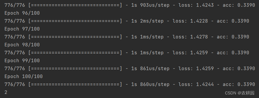
#神经网络配置好之后，就可以开始训练，拟合
logs=model.fit(age,fin_level, epochs=2000)  #进行匹配age和income，即训练，训练的次数为n次
#训练完之后，可以画个图看看
plt.scatter(logs.epoch, logs.history.get('loss'))

#训练完之后，就可以进行预测
#比如预测有20岁，他的财富等级能达到多少？
result=model.predict([20]) #这里必须是元组类型
# 预测结果：
print(int(result))

结果：

3.6 检查损失函数大小和准确率

#读入代码需要的库
import tensorflow as tf
import numpy as np
#把数据集读入，并拆分成训练集和测试集
def load_data(path):
    with np.load(path) as f:
        x_train, y_train = f['x_train'], f['y_train']
        x_test, y_test = f['x_test'], f['y_test']
        return (x_train, y_train), (x_test, y_test)
(x_train, y_train), (x_test, y_test) = load_data(path=r"C:\test\mnist.npz")  # mnist在本地的路径，需要自己替换
y_train

#数据预处理（进行归一化操作）
x_train = tf.keras.utils.normalize(x_train, axis=1)
x_test = tf.keras.utils.normalize(x_test, axis=1)

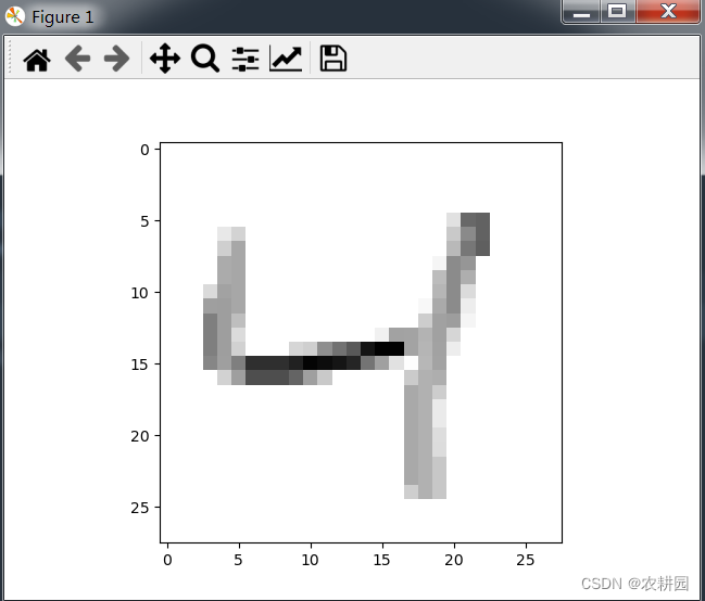
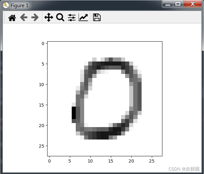
#数据预处理，查看一下数据集里的图片
import matplotlib.pyplot as plt
plt.imshow(x_train[2],cmap=plt.cm.binary)
plt.show()
print(y_train[2])

#建立模型，训练数据（每张图片的大小是28*28；神经网络有128层；最后要从0～9共10个数字中进行判断）
model = tf.keras.models.Sequential()
model.add(tf.keras.layers.Flatten(input_shape=(28,28)))
model.add(tf.keras.layers.Dense(128, activation=tf.nn.relu))
model.add(tf.keras.layers.Dense(128, activation=tf.nn.relu))
model.add(tf.keras.layers.Dense(10, activation=tf.nn.softmax))
model.compile(optimizer='adam',
              loss='sparse_categorical_crossentropy',
              metrics=['accuracy'])
model.fit(x_train, y_train, epochs=3)

#预测，并查看一下预测数据集的第一个数字是什么？并且用图形展示一下跟实际值对比
predictions = model.predict(x_test)
print(np.argmax(predictions[10]))
plt.imshow(x_test[10],cmap=plt.cm.binary)
plt.show()

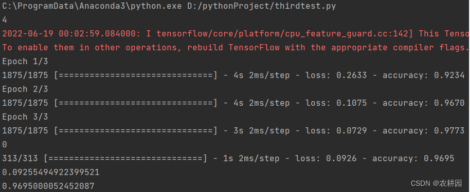
#检查损失函数大小和准确率
val_loss, val_acc = model.evaluate(x_test, y_test)
print(val_loss)
print(val_acc)

结果：

4 open cv

安装依赖包：
pip install opencv-python

AI小工具

https://huggingface.co/spaces/dalle-mini/dalle-mini
https://o9q981dirmk.typeform.com/to/zZtF1mVc?typeform-source=midjourney-gallery

4.1 读取图像

import cv2
print("版本："+str(cv2.__version__))
#人脸检测 方法：harr LBP
#机器学习算法：SVN 、KNN

#读取图像 image read
img=cv2.imread(r"C:\test\test.jpg")

#图片上画直线 cv2.line(图片，起点，终点，颜色,粗细)
cv2.line(img,(50,350),(250,450),(255,0,100),5)
#展示图片
cv2.imshow('test',img)
#创建窗口
cv2.namedWindow("test",0)
#调整大小
cv2.resizeWindow("test",800,600)
#等待消息相应
cv2.waitKey(0)
#释放窗口资源
cv2.destroyAllWindows()
#保存图片
cv2.imwrite(r"C:\test\test_bak.jpg",img)

注意：不能有中文的路径

4.2 转为灰度图像

import cv2
#载入图片
img = cv2.imread(r"C:\test\test.jpg")
#转为灰度图像
img_gray = cv2.cvtColor(img,cv2.COLOR_BGR2GRAY)
#展示已经载入的图像
cv2.imshow('img_gray',img_gray)
cv2.waitKey(0)
#对图像运用二值化处理
ret,thresh_img = cv2.threshold(img_gray,120,255,cv2.THRESH_BINARY_INV)
#展示二值化图像
#寻找二值图像的轮廓
contours,hierarchy = cv2.findContours(thresh_img,cv2.RETR_TREE,cv2.CHAIN_APPOX_SIMPLE)
#画轮廓
cv2.drawContours(img,contours,-1,(0,0,255),3)
#展示图像
cv2.imshow('img',img)
cv2.waitKey(0)
cv2.destoryAllWindows()

4.3 加马赛克

import cv2 #导入openCV库
import numpy as np #导入numpy库
img=cv2.imread(r"C:\test\test.jpg") #读取图片
imgInfo = img.shape
heigh = imgInfo[0]
width = imgInfo[1]
# m n 马赛克范围
for m in range(500,800):
    for n in range(500,800):
        if m%10 ==0 and n%10==0:
            # 小矩形块中，像素值的填充
            for i in range(0,10):
                for j in range(0,10):
                    (b,g,r) = img[m,n]
                    img[i+m,j+n] = (b,g,r)
cv2.imshow("dst",img)
cv2.waitKey(0)

4.4 训练模型

import tensorflow as tf
import numpy as np
#加载数据集
mnist=tf.keras.datasets.mnist

#指定输入数据的数组
input_xs=tf.keras.Input([28,28,1])

#拆分训练集和测试集
(x_train,y_train),(x_test,y_test)=mnist.load_data()

#构建待训练的神经网络模型
conv=tf.keras.layers.BatchNormalization()(input_xs)
conv=tf.keras.layers.Conv2D(filters=32, kernel_size=3, padding='SAME',activation=tf.nn.relu)(conv)
conv=tf.keras.layers.Conv2D(64, 3, padding='SAME',activation=tf.nn.relu)(conv)
conv=tf.keras.layers.MaxPool2D(strides=[1,1])(conv)
conv=tf.keras.layers.Conv2D(128, 3, padding='SAME',activation=tf.nn.relu)(conv)
#用于将输入层的数据压成一维的数据
flat=tf.keras.layers.Flatten()(conv)
#进入全连接层
dense=tf.keras.layers.Dense(512, activation=tf.nn.relu)(flat)
logits=tf.keras.layers.Dense(10, activation=tf.nn.softmax)(dense)

#主要做处理数据集
x_train,x_test=x_train/255.,x_test/255.
#1）用于给函数增加维度
x_train=tf.expand_dims(x_train,-1)
x_test=tf.expand_dims(x_test,-1)
x_train.shape

#2）把y类别标签转换为onehot编码
y_train=np.float32(tf.keras.utils.to_categorical(y_train,num_classes=10))
y_test=np.float32(tf.keras.utils.to_categorical(y_test,num_classes=10))
#3）设置数据批处理数
batch_size=512
#4）切分数据
train_dataset=tf.data.Dataset.from_tensor_slices((x_train,y_train)).batch(batch_size).shuffle(batch_size*10)
test_dataset=tf.data.Dataset.from_tensor_slices((x_test,y_test)).batch(batch_size)

#定义输入和输出的数据格式，并计算整个网络的参数信息
model=tf.keras.Model(inputs=input_xs, outputs=logits)
print(model.summary())
#定义网络损失函数
model.compile(optimizer=tf.optimizers.Adam(1e-3),
              loss=tf.losses.categorical_crossentropy,
              metrics=['accuracy'])
#开始训练模型
model.fit(train_dataset, epochs=3)

结果：

C:\ProgramData\Anaconda3\python.exe D:/test/Test.py
2022-06-19 16:13:25.195800: I tensorflow/core/platform/cpu_feature_guard.cc:142] This TensorFlow binary is optimized with oneAPI Deep Neural Network Library (oneDNN)to use the following CPU instructions in performance-critical operations:  AVX AVX2
To enable them in other operations, rebuild TensorFlow with the appropriate compiler flags.
2022-06-19 16:13:25.298800: W tensorflow/core/framework/cpu_allocator_impl.cc:81] Allocation of 191102976 exceeds 10% of free system memory.
2022-06-19 16:13:25.868800: W tensorflow/core/framework/cpu_allocator_impl.cc:81] Allocation of 191102976 exceeds 10% of free system memory.
2022-06-19 16:13:25.937800: W tensorflow/core/framework/cpu_allocator_impl.cc:81] Allocation of 191102976 exceeds 10% of free system memory.
Model: "functional_1"
_________________________________________________________________
Layer (type)                 Output Shape              Param #   
=================================================================
input_1 (InputLayer)         [(None, 28, 28, 1)]       0         
_________________________________________________________________
batch_normalization (BatchNo (None, 28, 28, 1)         4         
_________________________________________________________________
conv2d (Conv2D)              (None, 28, 28, 32)        320       
_________________________________________________________________
conv2d_1 (Conv2D)            (None, 28, 28, 64)        18496     
_________________________________________________________________
max_pooling2d (MaxPooling2D) (None, 27, 27, 64)        0         
_________________________________________________________________
conv2d_2 (Conv2D)            (None, 27, 27, 128)       73856     
_________________________________________________________________
flatten (Flatten)            (None, 93312)             0         
_________________________________________________________________
dense (Dense)                (None, 512)               47776256  
_________________________________________________________________
dense_1 (Dense)              (None, 10)                5130      
=================================================================
Total params: 47,874,062
Trainable params: 47,874,060
Non-trainable params: 2
_________________________________________________________________
None
2022-06-19 16:13:26.560800: W tensorflow/core/framework/cpu_allocator_impl.cc:81] Allocation of 376320000 exceeds 10% of free system memory.
2022-06-19 16:13:36.233800: W tensorflow/core/framework/cpu_allocator_impl.cc:81] Allocation of 376320000 exceeds 10% of free system memory.
Epoch 1/3
118/118 [==============================] - 571s 5s/step - loss: 0.2755 - accuracy: 0.9263
Epoch 2/3
118/118 [==============================] - 572s 5s/step - loss: 0.0414 - accuracy: 0.9874
Epoch 3/3
118/118 [==============================] - 559s 5s/step - loss: 0.0252 - accuracy: 0.9921

4.5 评估模型

import tensorflow as tf
import numpy as np
#加载数据集
mnist=tf.keras.datasets.mnist

#指定输入数据的数组
input_xs=tf.keras.Input([28,28,1])

#拆分训练集和测试集
(x_train,y_train),(x_test,y_test)=mnist.load_data()

#构建待训练的神经网络模型
conv=tf.keras.layers.BatchNormalization()(input_xs)
conv=tf.keras.layers.Conv2D(filters=32, kernel_size=3, padding='SAME',activation=tf.nn.relu)(conv)
conv=tf.keras.layers.Conv2D(64, 3, padding='SAME',activation=tf.nn.relu)(conv)
conv=tf.keras.layers.MaxPool2D(strides=[1,1])(conv)
conv=tf.keras.layers.Conv2D(128, 3, padding='SAME',activation=tf.nn.relu)(conv)
#用于将输入层的数据压成一维的数据
flat=tf.keras.layers.Flatten()(conv)
#进入全连接层
dense=tf.keras.layers.Dense(512, activation=tf.nn.relu)(flat)
logits=tf.keras.layers.Dense(10, activation=tf.nn.softmax)(dense)

#主要做处理数据集
x_train,x_test=x_train/255.,x_test/255.
#1）用于给函数增加维度
x_train=tf.expand_dims(x_train,-1)
x_test=tf.expand_dims(x_test,-1)
x_train.shape

#2）把y类别标签转换为onehot编码
y_train=np.float32(tf.keras.utils.to_categorical(y_train,num_classes=10))
y_test=np.float32(tf.keras.utils.to_categorical(y_test,num_classes=10))

#3）设置数据批处理数
batch_size=512

#4）切分数据
train_dataset=tf.data.Dataset.from_tensor_slices((x_train,y_train)).batch(batch_size).shuffle(batch_size*10)
test_dataset=tf.data.Dataset.from_tensor_slices((x_test,y_test)).batch(batch_size)

#定义输入和输出的数据格式，并计算整个网络的参数信息
model=tf.keras.Model(inputs=input_xs, outputs=logits)
print(model.summary())
#定义网络损失函数
model.compile(optimizer=tf.optimizers.Adam(1e-3),
              loss=tf.losses.categorical_crossentropy,
              metrics=['accuracy'])
#开始训练模型
model.fit(train_dataset, epochs=3)
#模型评估
score = model.evaluate(test_dataset)  # loss,accuracy
print('loss acc:', score)

5 工业应用

5.1 智能问答

file_name = 'know.pkl'
pkl_file = open(file_name,'rb')
my_data= pickle.load(pkl_file)
def my_know(ques,k_dict):
    return k_dict[ques],k_dict
print(my_know('你是谁',my_data))

5.2 展示盒图

import pandas as pd
import numpy as np
import matplotlib.pyplot as plt

#如果电脑加载某些库出现警告，可通过以下语句忽略警告
import warnings
warnings.filterwarnings("ignore")
#  数据读取
train_data = pd.read_table(r'E:\test\test_train.txt')
test_data = pd.read_table(r'E:\test\test_test.txt')

#数据预处理。查看缺失率，如果存在缺失值需要填补缺失值
print(train_data.isnull().sum())
#数据预处理，显示是否有缺失值情况以及各个变量的类型
print(train_data.info())
print(test_data.info())
# print(train_data.describe())

#数据预处理，仅仅把训练集划分特征与目标，为了后续绘图
train_data_X = train_data.drop(['target'], axis = 1)
train_data_y = train_data['target']

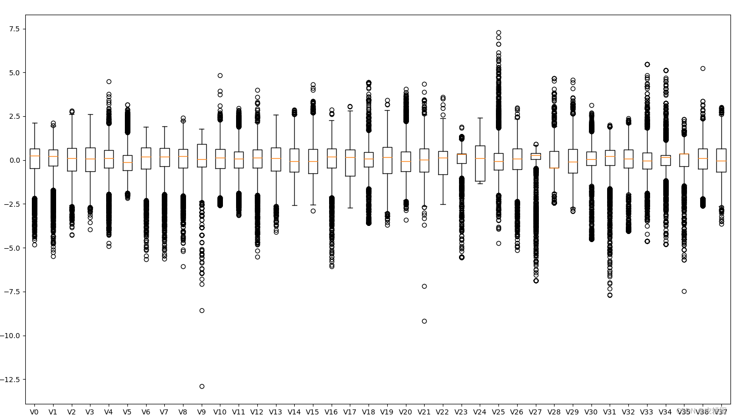
#数据预处理，通过盒图来观察数据集是否存在离散值（可视化观测）
data_all_X = pd.concat([train_data_X, test_data], axis=0)
plt.figure(figsize=(18,10))
plt.boxplot(x=data_all_X.values, labels=data_all_X.columns)
plt.show()

结果：

5.3 展示密度图

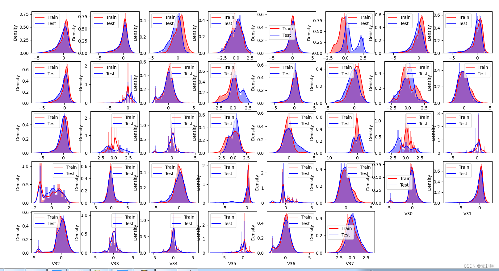
#数据预处理，根据盒图观察到的数据分布处理离散值，用均值替代它
train_data_X[train_data_X['V9']<=data_all_X['V9'].min()]=data_all_X['V9'].mean()
train_data_X[train_data_X['V21']<=data_all_X['V21'].min()]=data_all_X['V21'].mean()
train_data_X[train_data_X['V35']<=data_all_X['V35'].min()]=data_all_X['V35'].mean()
train_data_X[train_data_X['V37']>=data_all_X['V37'].max()]=data_all_X['V37'].mean()
#数据预处理，通过密度图来检查训练集和测试集数据分布差异（可视化观测）
import seaborn as sns
plt.figure(figsize=(30,30))
i = 1
for col in test_data.columns:
    plt.subplot(5,8,i)
    sns.distplot(train_data_X[col], color = 'red')
    sns.distplot(test_data[col], color = 'blue')
    plt.legend(['Train', 'Test'])
    i += 1

结果:

6 工业缺陷标注

6.1 标注工具label studio

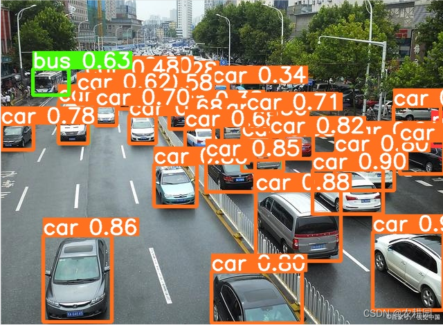
6.2 yolo的使用

import cv2
import numpy as np
#加载 yolo模型
from pygments.formatters import img

#加载需要预测的图像
img=cv2.imread(r"C:\test\21f.jpeg")

base= "D:\\test\\yolo\\"
net = cv2.dnn.readNet(base+"yolov3.weights",base+"yolov3.cfg")

#读入可检测的类别
classes=[]
with open(base+"coco.names") as f:
    classes=[line.strip() for line in f]
colors = np.random.uniform(0, 255, size=(len(classes), 3))
#可以自行查看检测类别清单
# print(len(classes),classes)

#图像预处理。这里的height、width等等，为了之后的画方框标出物体做准备
height,width,channel=img.shape
blob=cv2.dnn.blobFromImage(img,0.00392,(416,416),(0,0,0),True,crop=False)

#用yolo预测物体
net.setInput(blob)
layer_names = net.getLayerNames()
output_layers = [layer_names[i - 1] for i in net.getUnconnectedOutLayers()]
outs=net.forward(output_layers)
# print(outs)

#matplotlib
#inline
import matplotlib.pyplot as plt
# 画框
confidences = []
boxes = []
pred_indeces = []
# show info on pic
for out in outs:
    for detection in out:
        scores = detection[5:]
        pred_index = np.argmax(scores)
        confidence = scores[pred_index]

        if confidence > 0.5:
            center_x = int(detection[0] * width)
            center_y = int(detection[1] * height)
            w = int(detection[2] * width)
            h = int(detection[3] * height)
            # rectangle coordinates
            x = int(center_x - w / 2)
            y = int(center_y - h / 2)
            boxes.append([x, y, w, h])
            pred_indeces.append(pred_index)
            confidences.append(float(confidence))

# 剔除重复的框
indexes = cv2.dnn.NMSBoxes(boxes, confidences, 0.5, 0.5)

# 开始画框
font = cv2.FONT_HERSHEY_PLAIN
for i in range(len(boxes)):
    if i in indexes:
        x, y, w, h = boxes[i]
        label = classes[pred_indeces[i]]
        color = colors[i]
        cv2.rectangle(img, (x, y), (x + w, y + h), color, 2)
        cv2.putText(img, label, (x, y + 30), font, 1, color, 2)
cv2.imshow("detection", img)
cv2.waitKey(0)
# plt.show()

结果：

6.3 训练模型

#os.environ["CUDA_VISIBLE_DEVICES"] = "0"
from keras.callbacks import ModelCheckpoint
from keras.layers import Input, Conv2D, MaxPooling2D, UpSampling2D, Dropout
from keras.layers import concatenate
from keras.models import *
from keras.preprocessing.image import array_to_img
from tensorflow.keras.optimizers import Adam

from data import *

class myUnet(object):
   # 参数初始化定义
   def __init__(self, img_rows = 512, img_cols = 512):
      self.img_rows = img_rows
      self.img_cols = img_cols

   # 载入数据
   def load_data(self):
      mydata = dataProcess(self.img_rows, self.img_cols)
      imgs_train, imgs_mask_train = mydata.load_train_data()
      imgs_test = mydata.load_test_data()
      return imgs_train, imgs_mask_train, imgs_test

   def get_unet(self):
      inputs = Input((self.img_rows, self.img_cols,1))
      # 网络结构定义
      '''
      #unet with crop(because padding = valid) 

      conv1 = Conv2D(64, 3, activation = 'relu', padding = 'valid', kernel_initializer = 'he_normal')(inputs)
      print "conv1 shape:",conv1.shape
      conv1 = Conv2D(64, 3, activation = 'relu', padding = 'valid', kernel_initializer = 'he_normal')(conv1)
      print "conv1 shape:",conv1.shape
      crop1 = Cropping2D(cropping=((90,90),(90,90)))(conv1)
      print "crop1 shape:",crop1.shape
      pool1 = MaxPooling2D(pool_size=(2, 2))(conv1)
      print "pool1 shape:",pool1.shape

      conv2 = Conv2D(128, 3, activation = 'relu', padding = 'valid', kernel_initializer = 'he_normal')(pool1)
      print "conv2 shape:",conv2.shape
      conv2 = Conv2D(128, 3, activation = 'relu', padding = 'valid', kernel_initializer = 'he_normal')(conv2)
      print "conv2 shape:",conv2.shape
      crop2 = Cropping2D(cropping=((41,41),(41,41)))(conv2)
      print "crop2 shape:",crop2.shape
      pool2 = MaxPooling2D(pool_size=(2, 2))(conv2)
      print "pool2 shape:",pool2.shape

      conv3 = Conv2D(256, 3, activation = 'relu', padding = 'valid', kernel_initializer = 'he_normal')(pool2)
      print "conv3 shape:",conv3.shape
      conv3 = Conv2D(256, 3, activation = 'relu', padding = 'valid', kernel_initializer = 'he_normal')(conv3)
      print "conv3 shape:",conv3.shape
      crop3 = Cropping2D(cropping=((16,17),(16,17)))(conv3)
      print "crop3 shape:",crop3.shape
      pool3 = MaxPooling2D(pool_size=(2, 2))(conv3)
      print "pool3 shape:",pool3.shape

      conv4 = Conv2D(512, 3, activation = 'relu', padding = 'valid', kernel_initializer = 'he_normal')(pool3)
      conv4 = Conv2D(512, 3, activation = 'relu', padding = 'valid', kernel_initializer = 'he_normal')(conv4)
      drop4 = Dropout(0.5)(conv4)
      crop4 = Cropping2D(cropping=((4,4),(4,4)))(drop4)
      pool4 = MaxPooling2D(pool_size=(2, 2))(drop4)

      conv5 = Conv2D(1024, 3, activation = 'relu', padding = 'valid', kernel_initializer = 'he_normal')(pool4)
      conv5 = Conv2D(1024, 3, activation = 'relu', padding = 'valid', kernel_initializer = 'he_normal')(conv5)
      drop5 = Dropout(0.5)(conv5)

      up6 = Conv2D(512, 2, activation = 'relu', padding = 'same', kernel_initializer = 'he_normal')(UpSampling2D(size = (2,2))(drop5))
      merge6 = merge([crop4,up6], mode = 'concat', concat_axis = 3)
      conv6 = Conv2D(512, 3, activation = 'relu', padding = 'valid', kernel_initializer = 'he_normal')(merge6)
      conv6 = Conv2D(512, 3, activation = 'relu', padding = 'valid', kernel_initializer = 'he_normal')(conv6)

      up7 = Conv2D(256, 2, activation = 'relu', padding = 'same', kernel_initializer = 'he_normal')(UpSampling2D(size = (2,2))(conv6))
      merge7 = merge([crop3,up7], mode = 'concat', concat_axis = 3)
      conv7 = Conv2D(256, 3, activation = 'relu', padding = 'valid', kernel_initializer = 'he_normal')(merge7)
      conv7 = Conv2D(256, 3, activation = 'relu', padding = 'valid', kernel_initializer = 'he_normal')(conv7)

      up8 = Conv2D(128, 2, activation = 'relu', padding = 'same', kernel_initializer = 'he_normal')(UpSampling2D(size = (2,2))(conv7))
      merge8 = merge([crop2,up8], mode = 'concat', concat_axis = 3)
      conv8 = Conv2D(128, 3, activation = 'relu', padding = 'valid', kernel_initializer = 'he_normal')(merge8)
      conv8 = Conv2D(128, 3, activation = 'relu', padding = 'valid', kernel_initializer = 'he_normal')(conv8)

      up9 = Conv2D(64, 2, activation = 'relu', padding = 'same', kernel_initializer = 'he_normal')(UpSampling2D(size = (2,2))(conv8))
      merge9 = merge([crop1,up9], mode = 'concat', concat_axis = 3)
      conv9 = Conv2D(64, 3, activation = 'relu', padding = 'valid', kernel_initializer = 'he_normal')(merge9)
      conv9 = Conv2D(64, 3, activation = 'relu', padding = 'valid', kernel_initializer = 'he_normal')(conv9)
      conv9 = Conv2D(2, 3, activation = 'relu', padding = 'valid', kernel_initializer = 'he_normal')(conv9)
      '''

      conv1 = Conv2D(64, 3, activation = 'relu', padding = 'same', kernel_initializer = 'he_normal')(inputs)
      print ("conv1 shape:",conv1.shape)
      conv1 = Conv2D(64, 3, activation = 'relu', padding = 'same', kernel_initializer = 'he_normal')(conv1)
      print ("conv1 shape:",conv1.shape)
      pool1 = MaxPooling2D(pool_size=(2, 2))(conv1)
      print ("pool1 shape:",pool1.shape)

      conv2 = Conv2D(128, 3, activation = 'relu', padding = 'same', kernel_initializer = 'he_normal')(pool1)
      print ("conv2 shape:",conv2.shape)
      conv2 = Conv2D(128, 3, activation = 'relu', padding = 'same', kernel_initializer = 'he_normal')(conv2)
      print ("conv2 shape:",conv2.shape)
      pool2 = MaxPooling2D(pool_size=(2, 2))(conv2)
      print ("pool2 shape:",pool2.shape)

      conv3 = Conv2D(256, 3, activation = 'relu', padding = 'same', kernel_initializer = 'he_normal')(pool2)
      print ("conv3 shape:",conv3.shape)
      conv3 = Conv2D(256, 3, activation = 'relu', padding = 'same', kernel_initializer = 'he_normal')(conv3)
      print ("conv3 shape:",conv3.shape)
      pool3 = MaxPooling2D(pool_size=(2, 2))(conv3)
      print ("pool3 shape:",pool3.shape)

      conv4 = Conv2D(512, 3, activation = 'relu', padding = 'same', kernel_initializer = 'he_normal')(pool3)
      conv4 = Conv2D(512, 3, activation = 'relu', padding = 'same', kernel_initializer = 'he_normal')(conv4)
      drop4 = Dropout(0.5)(conv4)
      pool4 = MaxPooling2D(pool_size=(2, 2))(drop4)

      conv5 = Conv2D(1024, 3, activation = 'relu', padding = 'same', kernel_initializer = 'he_normal')(pool4)
      conv5 = Conv2D(1024, 3, activation = 'relu', padding = 'same', kernel_initializer = 'he_normal')(conv5)
      drop5 = Dropout(0.5)(conv5)

      up6 = Conv2D(512, 2, activation = 'relu', padding = 'same', kernel_initializer = 'he_normal')(UpSampling2D(size = (2,2))(drop5))
      # merge6 = merge([drop4,up6], mode = 'concat', concat_axis = 3)
      merge6 = concatenate([drop4, up6], axis=3)
      conv6 = Conv2D(512, 3, activation = 'relu', padding = 'same', kernel_initializer = 'he_normal')(merge6)
      conv6 = Conv2D(512, 3, activation = 'relu', padding = 'same', kernel_initializer = 'he_normal')(conv6)

      up7 = Conv2D(256, 2, activation = 'relu', padding = 'same', kernel_initializer = 'he_normal')(UpSampling2D(size = (2,2))(conv6))
      # merge7 = merge([conv3,up7], mode = 'concat', concat_axis = 3)
      merge7=concatenate([conv3,up7], axis=3)
      conv7 = Conv2D(256, 3, activation = 'relu', padding = 'same', kernel_initializer = 'he_normal')(merge7)
      conv7 = Conv2D(256, 3, activation = 'relu', padding = 'same', kernel_initializer = 'he_normal')(conv7)

      up8 = Conv2D(128, 2, activation = 'relu', padding = 'same', kernel_initializer = 'he_normal')(UpSampling2D(size = (2,2))(conv7))
      # merge8 = merge([conv2,up8], mode = 'concat', concat_axis = 3)
      merge8 = concatenate([conv2, up8], axis=3)
      conv8 = Conv2D(128, 3, activation = 'relu', padding = 'same', kernel_initializer = 'he_normal')(merge8)
      conv8 = Conv2D(128, 3, activation = 'relu', padding = 'same', kernel_initializer = 'he_normal')(conv8)

      up9 = Conv2D(64, 2, activation = 'relu', padding = 'same', kernel_initializer = 'he_normal')(UpSampling2D(size = (2,2))(conv8))
      # merge9 = merge([conv1,up9], mode = 'concat', concat_axis = 3)
      merge9 = concatenate([conv1, up9], axis=3)
      conv9 = Conv2D(64, 3, activation = 'relu', padding = 'same', kernel_initializer = 'he_normal')(merge9)
      conv9 = Conv2D(64, 3, activation = 'relu', padding = 'same', kernel_initializer = 'he_normal')(conv9)
      conv9 = Conv2D(2, 3, activation = 'relu', padding = 'same', kernel_initializer = 'he_normal')(conv9)
      conv10 = Conv2D(1, 1, activation = 'sigmoid')(conv9)

      model = Model(inputs = inputs, outputs = conv10)
      model.compile(optimizer = Adam(lr = 1e-4), loss = 'binary_crossentropy', metrics = ['accuracy'])
      return model

# 如果需要修改输入的格式，那么可以从以下开始修改，上面的结构部分不需要修改
   def train(self):
      print("loading data")
      imgs_train, imgs_mask_train, imgs_test = self.load_data()
      print("loading data done")
      model = self.get_unet()
      print("got unet")
      model_checkpoint = ModelCheckpoint('my_unet.hdf5', monitor='loss',verbose=1, save_best_only=True)
      print('Fitting model...')
      model.fit(imgs_train, imgs_mask_train, batch_size=2, epochs=10, verbose=1,validation_split=0.2, shuffle=True, callbacks=[model_checkpoint])

      print('predict test data')
      imgs_mask_test = model.predict(imgs_test, batch_size=1, verbose=1)
      np.save('../results/imgs_mask_test.npy', imgs_mask_test)

   def save_img(self):
      print("array to image")
      imgs = np.load('../results/imgs_mask_test.npy')
      for i in range(imgs.shape[0]):
         img = imgs[i]
         img = array_to_img(img)
         img.save("../results/%d.jpg"%(i))

if __name__ == '__main__':
   myunet = myUnet()
   myunet.train()
   myunet.save_img()

结果：

C:\ProgramData\Anaconda3\python.exe E:/test/unet.py
2022-06-28 00:14:05.242400: W tensorflow/stream_executor/platform/default/dso_loader.cc:64] Could not load dynamic library 'cudart64_110.dll'; dlerror: cudart64_110.dll not found
2022-06-28 00:14:05.386400: I tensorflow/stream_executor/cuda/cudart_stub.cc:29] Ignore above cudart dlerror if you do not have a GPU set up on your machine.
loading data
------------------------------
load train images...
------------------------------
------------------------------
load test images...
------------------------------
loading data done
2022-06-28 00:15:56.987400: W tensorflow/stream_executor/platform/default/dso_loader.cc:64] Could not load dynamic library 'cudart64_110.dll'; dlerror: cudart64_110.dll not found
2022-06-28 00:15:56.991400: W tensorflow/stream_executor/platform/default/dso_loader.cc:64] Could not load dynamic library 'cublas64_11.dll'; dlerror: cublas64_11.dll not found
2022-06-28 00:15:56.998400: W tensorflow/stream_executor/platform/default/dso_loader.cc:64] Could not load dynamic library 'cublasLt64_11.dll'; dlerror: cublasLt64_11.dll not found
2022-06-28 00:15:57.003400: W tensorflow/stream_executor/platform/default/dso_loader.cc:64] Could not load dynamic library 'cufft64_10.dll'; dlerror: cufft64_10.dll not found
2022-06-28 00:15:57.009400: W tensorflow/stream_executor/platform/default/dso_loader.cc:64] Could not load dynamic library 'curand64_10.dll'; dlerror: curand64_10.dll not found
2022-06-28 00:15:57.016400: W tensorflow/stream_executor/platform/default/dso_loader.cc:64] Could not load dynamic library 'cusolver64_11.dll'; dlerror: cusolver64_11.dll not found
2022-06-28 00:15:57.021400: W tensorflow/stream_executor/platform/default/dso_loader.cc:64] Could not load dynamic library 'cusparse64_11.dll'; dlerror: cusparse64_11.dll not found
2022-06-28 00:15:57.025400: W tensorflow/stream_executor/platform/default/dso_loader.cc:64] Could not load dynamic library 'cudnn64_8.dll'; dlerror: cudnn64_8.dll not found
2022-06-28 00:15:57.025400: W tensorflow/core/common_runtime/gpu/gpu_device.cc:1835] Cannot dlopen some GPU libraries. Please make sure the missing libraries mentioned above are installed properly if you would like to use GPU. Follow the guide at https://www.tensorflow.org/install/gpu for how to download and setup the required libraries for your platform.
Skipping registering GPU devices...
2022-06-28 00:15:57.087400: I tensorflow/core/platform/cpu_feature_guard.cc:142] This TensorFlow binary is optimized with oneAPI Deep Neural Network Library (oneDNN) to use the following CPU instructions in performance-critical operations:  AVX AVX2
To enable them in other operations, rebuild TensorFlow with the appropriate compiler flags.
conv1 shape: (None, 512, 512, 64)
conv1 shape: (None, 512, 512, 64)
pool1 shape: (None, 256, 256, 64)
conv2 shape: (None, 256, 256, 128)
conv2 shape: (None, 256, 256, 128)
pool2 shape: (None, 128, 128, 128)
conv3 shape: (None, 128, 128, 256)
conv3 shape: (None, 128, 128, 256)
pool3 shape: (None, 64, 64, 256)
C:\ProgramData\Anaconda3\lib\site-packages\keras\optimizer_v2\optimizer_v2.py:355: UserWarning: The `lr` argument is deprecated, use `learning_rate` instead.
  warnings.warn(
got unet
Fitting model...
2022-06-28 00:16:10.424400: I tensorflow/compiler/mlir/mlir_graph_optimization_pass.cc:185] None of the MLIR Optimization Passes are enabled (registered 2)
Epoch 1/10
2022-06-28 00:16:21.882400: W tensorflow/core/framework/cpu_allocator_impl.cc:80] Allocation of 603979776 exceeds 10% of free system memory.
2022-06-28 00:16:21.991400: W tensorflow/core/framework/cpu_allocator_impl.cc:80] Allocation of 603979776 exceeds 10% of free system memory.
2022-06-28 00:16:22.440400: W tensorflow/core/framework/cpu_allocator_impl.cc:80] Allocation of 603979776 exceeds 10% of free system memory.
2022-06-28 00:16:22.441400: W tensorflow/core/framework/cpu_allocator_impl.cc:80] Allocation of 603979776 exceeds 10% of free system memory.
2022-06-28 00:16:23.503400: W tensorflow/core/framework/cpu_allocator_impl.cc:80] Allocation of 1207959552 exceeds 10% of free system memory.
12/12 [==============================] - 1102s 33s/step - loss: 0.5296 - accuracy: 0.7536 - val_loss: 0.4899 - val_accuracy: 0.7535

Epoch 00001: loss improved from inf to 0.52965, saving model to my_unet.hdf5
Epoch 2/10
12/12 [==============================] - 346s 29s/step - loss: 0.4077 - accuracy: 0.7870 - val_loss: 0.4166 - val_accuracy: 0.7539

Epoch 00002: loss improved from 0.52965 to 0.40774, saving model to my_unet.hdf5
Epoch 3/10
12/12 [==============================] - 345s 29s/step - loss: 0.3681 - accuracy: 0.7871 - val_loss: 0.3971 - val_accuracy: 0.7540

Epoch 00003: loss improved from 0.40774 to 0.36815, saving model to my_unet.hdf5
Epoch 4/10
12/12 [==============================] - 345s 29s/step - loss: 0.3405 - accuracy: 0.7871 - val_loss: 0.3984 - val_accuracy: 0.7540

Epoch 00004: loss improved from 0.36815 to 0.34047, saving model to my_unet.hdf5
Epoch 5/10
12/12 [==============================] - 343s 29s/step - loss: 0.3427 - accuracy: 0.7873 - val_loss: 0.4047 - val_accuracy: 0.7539

Epoch 00005: loss did not improve from 0.34047
Epoch 6/10
12/12 [==============================] - 345s 29s/step - loss: 0.3317 - accuracy: 0.8290 - val_loss: 0.3783 - val_accuracy: 0.8346

Epoch 00006: loss improved from 0.34047 to 0.33174, saving model to my_unet.hdf5
Epoch 7/10
12/12 [==============================] - 344s 29s/step - loss: 0.3285 - accuracy: 0.8635 - val_loss: 0.3735 - val_accuracy: 0.8447

Epoch 00007: loss improved from 0.33174 to 0.32846, saving model to my_unet.hdf5
Epoch 8/10
12/12 [==============================] - 345s 29s/step - loss: 0.3154 - accuracy: 0.8660 - val_loss: 0.3599 - val_accuracy: 0.8284

Epoch 00008: loss improved from 0.32846 to 0.31544, saving model to my_unet.hdf5
Epoch 9/10
12/12 [==============================] - 345s 29s/step - loss: 0.2928 - accuracy: 0.8714 - val_loss: 0.3241 - val_accuracy: 0.8538

Epoch 00009: loss improved from 0.31544 to 0.29277, saving model to my_unet.hdf5
Epoch 10/10
12/12 [==============================] - 347s 29s/step - loss: 0.2814 - accuracy: 0.8749 - val_loss: 0.3226 - val_accuracy: 0.8524

Epoch 00010: loss improved from 0.29277 to 0.28143, saving model to my_unet.hdf5
predict test data
30/30 [==============================] - 140s 3s/step
array to image

进程已结束，退出代码为 0

6.4 预测

from unet import *
from data import *
import matplotlib.pyplot as plt
import numpy as np

xaxis().set_visible(False)
print("array to image")
imgs = np.load('../results/imgs_mask_test.npy')
for i in range(imgs.shape[0]):
    img = imgs[i]
    img = array_to_img(img)
    img.save("../results/%d.jpg" % (i))

结果：

C:\ProgramData\Anaconda3\python.exe E:/test/test_predict.py
2022-06-28 01:46:23.331400: W tensorflow/stream_executor/platform/default/dso_loader.cc:64] Could not load dynamic library 'cudart64_110.dll'; dlerror: cudart64_110.dll not found
2022-06-28 01:46:23.331400: I tensorflow/stream_executor/cuda/cudart_stub.cc:29] Ignore above cudart dlerror if you do not have a GPU set up on your machine.
array to image

进程已结束，退出代码为 0

7 视觉和图像

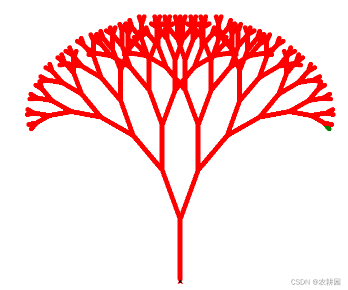
7.1 绘制树枝

import turtle
def draw_branch(length):
    #绘制右侧树枝
    if length >5:
        if length ==10:
            turtle.pencolor('green')
        turtle.forward(length)
        turtle.right(20)
        draw_branch(length-15)
        #绘制左侧树枝
        turtle.left(40)
        draw_branch(length-15)
        #返回之前树枝
        turtle.right(20)
        turtle.backward(length)
        if length==10:
            turtle.pencolor('yellow')
        else:
            turtle.pencolor('red')
def main():
    turtle.pencolor('green')
    turtle.pensize(10)
    turtle.left(90)
    turtle.penup()
    turtle.backward(160)
    turtle.pendown()
    draw_branch(120)
    turtle.exitonclick()
if __name__== '__main__':
    main()

结果：

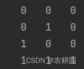
7.2 逻辑运算

1、定义x1,x2作为数组
2、定义w1,w2作为数组
3、定义阈值b
4、计算y，如y=x*w+b
5、把y和0做判断，得到最后y的取值
6、打印结果

import numpy as np
def AND(x1,x2):
    x=np.array([x1,x2])
    w=np.array([0.5,0.5])
    b = -0.7
    y=np.sum(x*w)+b
    if y<=0:
        return 0
    else:
        return 1
for x1 in range(2):
    for x2 in range(2):
        print("{0:3d} {1:3d} {2:3d}".format(x1,x2,AND(x1,x2)))

结果：

7.3 yolov5

下载地址：https://github.com/ultralytics/yolov5

7.3.1 安装相应的依赖包

下载到本地后，进行安装相应的依赖（用douban提高下载速度）

pip install  -i http://pypi.douban.com/simple/ --trusted-host=pypi.douban.com/simple  -r  E:\test\yolov5-master\requirements.txt

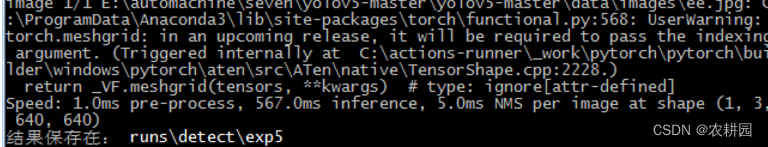
7.3.2 处理视频

python D:\test\yolov5-master\detect.py --source D:\test\yolov5-master\mp_vedio\v_test.mp4 --weights yolov5s.pt

结果：

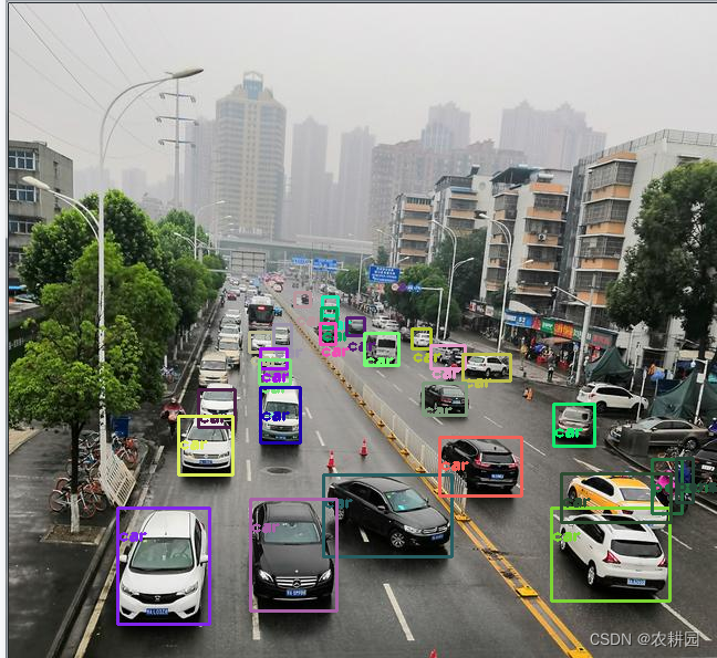
7.3.3 处理图片

python  detect.py  --source  D:\test\animals.jpg    --weight yolov5s.pt

结果：

7.3.4 训练模型

第一步：设置标注工具labelImg为yolo格式
第二步：标注图片（标注的图片越多越准确）
第三步：训练模型

python train.py --cfg D:\test\yolov5-master\models\yolov5sxiugai.yaml --data D:\test\my_datasets\lfy_test.yaml

第四步：检测模型的正确率

8 常用机器学习平台

alteryx
参考地址：https://www.alteryx.com/

阿里云机器学习平台PAI（阿里云）
参考地址：https://www.aliyun.com/product/bigdata/learn

Amazon SageMaker（aws）
参考地址：https://aws.amazon.com/cn/campaigns/sagemaker/?sc_channel=PS&sc_campaign=acquisition_CN&sc_publisher=baidu&sc_category=pc&sc_medium=%E5%93%81%E7%89%8C%E4%BA%A7%E5%93%81_%E6%9C%BA%E5%99%A8%E5%AD%A6%E4%B9%A0_SageMaker_b&sc_content=%E6%9C%BA%E5%99%A8%E5%AD%A6%E4%B9%A0_SageMaker_%E7%B2%BE&sc_detail=aws%20SageMaker&sc_segment=JK-AWS%20b4&sc_matchtype=exact&sc_country=CN&s_kwcid=AL!4422!88!48220743151!!232620117750&ef_id=YszhpwAABF9syFY9:20220712025119:s

百度飞浆 BML（百度智能云）
参考地址：https://ai.baidu.com/bml/?track=cp:aipinzhuan|pf:pc|pp:BML|pu:title|ci:|kw:10515737

邦盛科技智能学习平台（邦盛科技）
参考地址：https://www.bsfit.com.cn/product#Product-machine-learning

创新奇智Orion分布式机器学习平台（创新奇智）
参考地址：https://www.ainnovation.com/mmo/orion

DataCanvas APS机器学习平台（DataCanvas）
参考地址：https://www.datacanvas.com/product-aps

第四范式先知平台（4Paradigm）
参考地址：https://www.4paradigm.com/

Google Cloud AutoML（Google Cloud）
参考地址：https://cloud.google.com/automl/

华为ModelArts（HUAWEI）
参考地址：https://www.huaweicloud.com/

IBM Watson Studio（IBM）
参考地址：https://www.ibm.com/cloud/watson-studio

京东 NeuFoundry（京东云）
参考地址：https://www.jdcloud.com/cn/solutions/neufoundry