题目:SPINN: Synergistic Progressive Inferenceof Neural Networks over Device and Cloud
SPINN:设备和云上神经网络的协同渐进推理
作者:Stefanos Laskaridis , Stylianos I. Venieris ,Mario Almeida , Ilias Leontiadis ,
Nicholas D. Lane
摘要:Despite the soaring use of convolutional neural networks (CNNs) in mobile applications, uniformly sustaining high-performance inference on mobile has been elusive due to the excessive computational demands of modern CNNs and the increasing diversity of deployed devices. A popular alternative comprises offloading CNN processing to powerful cloud-based servers. Nevertheless, by relying on the cloud to produce outputs, emerging mission-critical and high-mobility applications, such as drone obstacle avoidance or interactive applications, can suffer from the dynamic connectivity conditions and the uncertain availability of the cloud. In this paper, we propose SPINN, a distributed inference system that employs synergistic device-cloud computation together with a progressive inference method to deliver fast and robust CNN inference across diverse settings. The proposed system introduces a novel scheduler that co-optimises the early-exit policy and the CNN splitting at run time, in order to adapt to dynamic conditions and meet user-defined service-level requirements. Quantitative evaluation illustrates that SPINN outperforms its state-of-the-art collaborative inference counterparts by up to 2× in achieved throughput under varying network conditions, reduces the server cost by up to 6.8× and improves accuracy by 20.7% under latency constraints, while providing robust operation under uncertain connectivity conditions and significant energy savings compared to cloud-centric execution.
尽管卷积神经网络在移动设备中的使用激增,但由于现代CNN过量的计算需求和日益多样化的部署设备,在移动应用上保持高性能推理一直难以实现。一个流行的替代方案是将CNN处理卸载到强大的基于云的服务器上。然而,由于依赖云产生输出,新兴的任务关键型和高移动型应用程序,如无人机避障或交互式应用程序,可能会受到动态连接条件和云可用性不确定的影响。在本文中,我们提出了SPINN,一个分布式推理系统,它协同设备和云共同计算并使用渐进推理方法,在不同的设置下提供快速和鲁棒的CNN推理。我们提出的系统引入了一个新的调度程序,在运行时联合优化早期退出策略和CNN拆分,以适应动态条件和满足用户定义的服务水平需求。定量评估表明,在不同的网络条件下,SPINN比其最先进的协作推理对手的吞吐量高出2倍,减少服务器成本高达6.8倍,并在延迟约束下提高20.7%的准确率。同时,与以云为中心的执行相比,可以在不确定的连接条件下提供可靠的操作,并显著节省能源。
KEYWORDS:Deep neural networks, distributed systems, mobile computing
关键词:深度神经网络、分布式系统、移动计算
一、介绍
With the spectrum of CNN-driven applications expanding rapidly, their deployment across mobile platforms poses significant challenges. Modern CNNs [20, 68] have excessive computational demands that hinder their wide adoption in resource-constrained mobile devices. Furthermore, emerging user-facing [80] and mission-critical [37,42,66] CNN applications require low-latency processing to ensure high quality of experience (QoE) [4] and safety [11].
随着cnn驱动的应用程序的快速扩展,它们在移动平台上的部署带来了巨大的挑战。现代CNN[20,68]有过大的计算需求,这阻碍了它们在资源受限的移动设备上的广泛应用。此外,新兴的面向用户型[80]和任务关键型[37,42,66]CNN的应用需要低延迟处理,以确保高质量的体验(QoE)[4]和安全[11]。
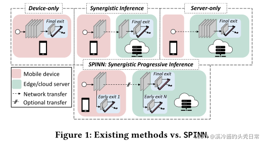
Given the recent trend of integrating powerful System-on-Chips (SoCs) in consumer devices [2, 25, 78], direct on-device CNN execution is becoming possible (Figure 1 - top left). Nevertheless,while flagship devices can support the performance requirements of CNN workloads, the current landscape is still very diverse, including previous-gen and low-end models [80]. In this context, the less powerful low-tier devices struggle to consistently meet the application-level performance needs [2]
鉴于最近在消费设备中集成强大的片上系统(Soc)的趋势[2,25,78],直接在设备上执行CNN正成为可能(图1 -左上角)。然而,旗舰设备可以在可以支持CNN工作量的性能需求,但目前的形势仍然非常多样化,包括上一代和低端型号[80]。在这种情况下,功能较弱的底层设备很难始终满足应用程序级的性能需求。
As an alternative, service providers typically employ cloud-centric solutions (Figure 1 - top right). With this setup, inputs collected by mobile devices are transmitted to a remote server to perform CNN inference using powerful accelerators [3, 6, 12, 19, 31, 32]. However, this extra computation capability comes at a price. First, cloud execution is highly dependent on the dynamic network conditions, with performance dropping radically when the communication channel is degraded. Second, hosting resources capable of accelerating machine learning tasks comes at a significant cost [40]. Moreover, while public cloud providers offer elastic cost scaling,
there are also privacy and security concerns [64].
作为替代方案,服务提供商通常采用以云为中心的解决方案(图1 -右上角)。通过这种设置,移动设备收集的输入信息被传输到远程服务器,使用强大的加速器执行CNN推断[3,6,12,19,31,32]。然而,这种额外的计算能力是有代价的。首先,云执行高度依赖于动态网络条件,当通信通道降级时,性能会急剧下降。其次,能够加速机器学习任务的托管资源成本很高。此外,在公共云提供商提供弹性成本伸缩的同时,也存在隐私和安全问题[64]。
To address these limitations, a recent line of work [22, 34, 46] has proposed the collaboration between device and cloud for CNN inference (Figure 1 - top center). Such schemes typically treat the CNN as a computation graph and partition it between device and cloud. At run time, the client executes the first part of the model and transmits the intermediate results to a remote server. The server continues the model execution and returns the final result back to the device. Overall, this approach allows tuning the fraction of the CNN that will be executed on each platform based on their capabilities.
为了解决这些限制,最近的工作[22,34,46]提出了在CNN推理中实现设备和云之间的协作(图1 的顶部中心)。这种方案通常将CNN视为一个计算图,并将其划分到设备和云中。在运行时,客户机执行模型的第一部分,并将中间结果传输到远程服务器。服务器继续模型执行并将最终结果返回给设备。总的来说,这种方法允许根据每个平台的能力来调整将在每个平台上执行的CNN比例。
Despite their advantages, existing device-cloud collaborative inference solutions suffer from a set of limitations. First, similar to cloud execution, the QoE is greatly affected by the network conditions as execution can fail catastrophically when the link is severely deteriorated. This lack of network fault tolerance also prevents the use of more cost-efficient cloud solutions, e.g. using ephemeral spare cloud resources at a fraction of the price.1Furthermore, CNNs are increasingly deployed in applications with stringent demands across multiple dimensions (e.g. target latency, throughput and accuracy, or device and cloud costs).2Existing collaborative methods cannot sufficiently meet these requirements.
尽管现有的设备云协作推断解决方案有其优点,但它们也存在一系列的局限性。首先,与云执行类似,QoE(用户体验质量)受到网络条件的很大影响,当链接严重恶化时,执行可能会灾难性地失败。这种网络容错能力的缺乏也阻止了更经济有效的云解决方案的使用,例如以极低的价格使用临时的备用云资源。此外,cnn越来越多地部署在对多个维度(例如目标延迟、吞吐量和准确性,或设备和云成本)有严格要求的应用程序中。现有的协作方法不能充分满足这些需求。
To this end, we present SPINN, a distributed system that enables robust CNN inference in highly dynamic environments, while meeting multi-objective application-level requirements (SLAs). This is accomplished through a novel scheduler that takes advantage of progressive inference; a mechanism that allows the system to exit early at different parts of the CNN during inference, based on the input complexity (Figure 1 - bottom). The scheduler optimises the
overall execution by jointly tuning both the split point selection and the early-exit policy at run time to sustain high performance and meet the application SLAs under fluctuating resources (e.g. net-
work speed, device/server load). The guarantee of a local early exit renders server availability non-critical and enables robust operation even under uncertain connectivity. Overall, this work makes the following key contributions:
SLAs:Service Level Agreements 服务水平协议
为此,我们提出了SPINN,这是一个分布式系统,能够在高度动态的环境中进行健壮的CNN推断,同时满足多目标应用程序级需求(SLAs)。这是通过一个新颖的调度程序实现的,它利用了渐进推理:一种基于复杂性输入的机制,允许系统在推理过程中在CNN的不同部分早期退出(图1 -下)。调度器通过在运行时联合调优分离点选择和早期退出策略来优化整体执行,以保持高性能,并在资源(如网络速度、设备/服务器负载)波动的情况下满足应用程序的SLAs。本地早期退出的保证使服务器可用性变得不重要,并且即使在不确定的连接下也能实现健壮的操作。总的来说,这项工作有以下主要贡献:
A progressive inference mechanism that enables the fast and reliable execution of CNN inference across device and cloud. Concretely, on top of existing early-exit designs, we propose an early-exit-aware cancellation mechanism that allows the interruption of the (local/remote) inference when having a confident early prediction, thus minimising redundant computation and
transfers during inference. Simultaneously, reflecting on the un- certain connectivity of mobile devices we design an early-exit scheme with robust execution in mind, even under severe connectivity disruption or cloud unavailability. By carefully placing the early exits in the backbone network and allowing for graceful fallback to locally available results, we guarantee the responsive-ness and reliability of the system and overcome limitations of existing offloading systems.
一种渐进的推理机制,能够跨设备和云快速可靠地执行CNN推理。具体地说,在现有的早期退出设计的基础上,我们提出了一种早期退出感知的取消机制,允许在有一个自信的早期预测时中断(本地/远程)推断,从而最大限度地减少推理过程中的冗余计算和传输。同时,考虑到移动设备的不确定连接性,我们设计的提前退出的方案还考虑到了执行的稳定性,即使在严重的连接性中断或云不可用的情况下。通过在骨干网络中放置早期出口,并允许很好的回退到本地可用的结果,我们保证了系统的响应性和可靠性,并克服了现有卸载系统的限制。
A CNN-specific packing mechanism that exploits the reduced-precision resilience and sparsity of CNN workloads to minimise transfer overhead. Our communication optimiser combines a lossless and an accuracy-aware lossy compression component which exposes previously unattainable designs for collaborative inference, while not sacrificing the end accuracy of the system.
一种特定于CNN的封装机制,利用CNN工作负载的降低精度的弹性和稀疏性来最小化传输开销。我们的通信优化器结合了一个无损和一个精度感知的有损压缩组件,它展示了以前无法实现的协作推理设计,同时不牺牲系统的最终精度。
An SLA- and condition-aware scheduler that co-optimises i) the early-exit policy of progressive CNNs and ii) their partitioning between device and cloud at run time. The proposed scheduler employs a multi-objective framework to capture the user-defined importance of multiple performance metrics and translate them into SLAs. Moreover, by surveilling the volatile network conditions and resources load at run time, the scheduler dynamically selects the configuration that yields the highest performance by taking into account contextual runtime information and feedback from previous executions.
一个SLA和条件感知的协同优化的调度程序:1)渐进式CNN的提前退出策略。2)它们在运行时在设备和云之间的分区。提出的调度器使用一个多目标框架来捕获用户定义的多个性能指标的重要性,并将它们转换为SLAs。此外,通过在运行时监视不稳定的网络条件和资源负载,调度器通过考虑上下文运行时信息和以前执行的反馈,动态地选择产生最高性能的配置。
二、背景和相关工作
To optimise the execution of CNN workloads, several solutions have been proposed, from compiler [1, 30, 65] and runtime optimisations [36, 43, 49] to custom cloud [7, 19, 34] and accelerator designs [75, 79]. While these works target a single model withdevice- or cloud-only execution, the increased computational capabilities of client devices [2, 25] have led to schemes that maximise performance via device-cloud synergy. Next, we outline significant work in this direction and visit approximate computing alternatives which exploit accuracy-latency trade-offs during inference.
为了优化CNN工作负载的执行,已经提出了几种解决方案,从编译器[1,30,65]和运行时优化[36,43,49]到定制云[7,19,34]和加速器设计[75,79]。然而,这些工作的目标是单一的模型,只有设备或云执行,但客户端设备计算能力的增加[2,25]已经导致了通过设备-云协同是实现性能最大化的方案。接下来,我们概述了这个方向的重要工作,并研究了在推断过程中利用精度-延迟权衡的近似计算方案。
Approximate Inference.In applications that can tolerate some accuracy drop, a line of work [9, 18, 45] exploits the accuracy-latency trade-off through various techniques. In particular , NestDNN [9] employs a multi-capacity model that incorporates multiple descendant (i.e. pruned) models to expose an accuracy-complexity trade-off mechanism. However, such models cannot be natively split between device and cloud. On the other hand, model selection systems [18, 45] employ multiple variants of a single model (e.g. quantised, pruned) with different accuracy-latency trade-offs. At run time, they choose the most appropriate variant based on the application requirements and determine where it will be executed. Similarly, classifier cascades [21, 33, 38, 39, 71] require multiple models to obtain performance gains. Despite the advantages of both, using multiple models adds substantial overhead in terms of maintenance, training and deployment.
近似推理。在某些可以容忍精度下降的应用程序中,一行工作[9,18,45]通过各种技术实现精度-延迟的权衡。具体来说,NestDNN[9]使用了一个多容量模型,该模型包含多个后代(即修剪过的)模型,以实现准确性-复杂性权衡机制。然而,这样的模型不能在设备和云之间分割。另一方面,模型选择系统[18,45]使用单个模型的多个变体(如量化的、修剪的),具有不同的精度-延迟权衡。在运行时,他们根据应用程序需求选择最合适的变体,并决定在哪里执行它。类似地,分类器级联[21,33,38,39,71]需要多个模型来获得性能增益。尽管这两种模型都有优势,但使用多个模型在维护、培训和部署方面增加了大量开销。
Progressive Inference Networks. A growing body of work from both the research [23, 35, 72, 81, 84] and industry communities [55, 74] has proposed transforming a given model into a progressive inference network by introducing intermediate exits throughout its depth. By exploiting the different complexity of incoming samples, easier examples can early-exit and save on further computations. So far, existing works have mainly explored the hand-crafted design of early-exit architectures (MSDNet [23],SCAN [84]), the platform- and SLA-agnostic derivation of early-exit networks from generic models (BranchyNet [72], SDN [35]) or the hardware-aware deployment of such networks (HAPI [44]). Despite the recent progress, these techniques have not capitalised upon the unique potential of such models to yield high mobile performance through distributed execution and app-tailored early-exiting. In this context, SPINN is the first progressive inference approach equipped with a principled method of selectively splitting execution between device and server, while also tuning the early-exit policy, enabling high performance across dynamic settings.
渐进的推理网络。研究[23,35,72,81,84]和产业界[55,74]有越来越多的工作提出,通过在模型的深度中引入中间出口,将给定的模型转化为渐进推理网络。通过利用传入样本不同的复杂性,更简单实现提前退出并节省进一步的计算。到目前为止,现有的工作主要探索了早期退出架构的人工设计(MSDNet [23], SCAN[84]),早期退出网络的平台和与SLAs无关的衍生(BranchyNet [72], SDN[35])或此类网络的硬件感知部署(HAPI[44])。尽管最近取得了进展,但这些技术并没有充分利用这些模型的独特潜力,没有通过分布式执行和应用程序定制的早期退出来实现高移动性能。在本文中,SPINN是第一种渐进推理方法,它具有选择性地在设备和服务器之间分割执行原则的方法,同时还调优早期退出策略,从而实现跨动态设置的高性能。
Device-Cloud Synergy for CNN Inference. To achieve efficient CNN processing, several works have explored collaborative computation over device, edge and cloud. One of the most prominent pieces of work, Neurosurgeon [34], partitions the CNN between a device-mapped head and a cloud-mapped tail and selects a single split point based on the device and cloud load as well as the network conditions. Similarly, DADS [22] tackles CNN offloading, but from a scheduler-centric standpoint, with the aim to yield the optimal partitioning scheme in the case of high and low server load. However, both systems only optimise for single-criterion objectives (latency or energy consumption), they lack support for app-specific SLAs, and suffer catastrophically when the remote server is unavailable. With a focus on data transfer, JALAD [47] incorporates lossy compression to minimise the offload transmission overhead. Nevertheless, to yield high performance, the proposed system sacrifices substantial accuracy (i.e. >5%).JointDNN [8] modelled CNN offloading as a graph split problem, but targets only offline scheduling and static environments instead of highly dynamic mobile settings. Contrary to these systems, SPINN introduces a novel scheduler that adapts the execution to the dynamic contextual conditions and jointly tunes the offloading point and early-exit policy to meet the application-level requirements. Moreover, by guaranteeing the presence of a local result, SPINN provides resilience to server disconnections.
CNN推理的设备-云协同。为了实现高效的CNN处理,一些研究已经探索了在设备、边缘和云上的协同计算。最突出的工作之一是神经外科医生[34],将CNN划分为设备映射的头部和云映射的尾部,并根据设备和云负载以及网络条件选择单个分裂点。类似地,DADS[22]处理CNN卸载,但是从调度中心的角度出发,目的是在服务器负载高和低的情况下生成最优的分区方案。然而,这两个系统都只针对单一标准目标(延迟或能耗)进行优化,它们缺乏对特定于应用程序的SLAs的支持,并且在远程服务器不可用时遭受灾难性的损失。针对数据传输,JALAD[47]采用了有损压缩,以最大限度地减少传输开销。然而,为了获得高性能,所提出的系统牺牲了大量的准确性(即>5%)。JointDNN[8]将CNN卸载建模为一个图分割问题,但只针对离线调度和静态环境,而不是高度动态的移动设置。与这些系统相反,SPINN引入了一种新的调度器,它使执行适应动态环境条件,并联合调优卸载点和早期退出策略,以满足应用程序级需求。此外,通过保证本地结果的存在,SPINN提供了对服务器断开的弹性。
Apart from offloading CNNs to a dedicated server, a number of works have focused on tangential problems. IONN [29] tackles a slightly different problem, where instead of preinstalling the CNN model to a remote machine, the client device can offload to any close-by server by transmitting both the incoming data and the model in a shared-nothing setup. Simultaneously, various works [50, 51, 85] have examined the case where the client device can offload to other
devices in the local network. Last, [73] also employs cloud-device synergy and progressive inference, but with a very different focus, i.e. to perform joint classification from a multi-view, multi-camera standpoint. Its models, though, are statically allocated to devices and its fixed, statically-defined early-exit policy, renders it impractical for dynamic environments.
除了将CNN卸载到专用服务器之外,许多工作都集中在一些无关紧要的问题上。IONN[29]解决了一个稍微不同的问题,它不是将CNN模型预先安装到远程机器上,而是客户端设备可以通过在无共享设置中传输传入数据和模型,将其卸载到任何附近的服务器上。同时,各种工作[50,51,85]已经提出了客户机设备可以卸载到本地网络中的其他设备的情况。最后,[73]也采用了云设备协同和渐进推理,但重点非常不同,即从多视角、多摄像机的角度进行联合分类。然而,它的模型是静态分配给设备的,它的固定的、静态定义的早期退出策略使得它在动态环境中不可行。
Offloading Multi-exit Models.Closer to our approach,Edgent [46] proposes a way of merging offloading with multi-exit models. Nonetheless, this work has several limitations. First, the inference workflow disregards data locality and always starts from the cloud.Consequently, inputs are always transmitted, paying an additional transfer cost. Second, early-exit networks are not utilised with progressive inference, i.e. inputs do not early-exit based on their complexity. Instead, Edgent tunes the model’s complexity by selecting a single intermediary exit for all inputs. Therefore, the end system does not benefit from the variable complexity of inputs. Finally, the system has been evaluated solely on simple models (AlexNet) and datasets (CIFAR-10), less impacted by low-latency or unreliable network conditions. In contrast, SPINN exploits the fact that data already reside on the device to avoid wasteful input transfers, and employs a CNN-tailored technique to compress the offloaded data. Furthermore, not only our scheduler supports additional optimisation objectives, but it also takes advantage of the input’s complexity to exit early, saving resource usage with minimal impact on accuracy.
卸载多出口模型。与我们的方法很接近的是Edgent[46],它提出了一种将卸载与多出口模型合并的方法。然而,这项工作有几个局限性。首先,推理工作流忽略了数据的局部性,总是从云开始。因此,输入总是被传输,支付额外的转移成本。第二,早期退出网络没有被用于渐进推理,也就是说,基于其复杂性,输入不会早期退出。相反,Edgent通过为所有输入选择一个中间出口来调整模型的复杂性。因此,终端系统不能从输入的可变复杂性中获益。最后,该系统仅在简单模型(AlexNet)和数据集(CIFAR-10)上进行了评估,较少受到低延迟或不可靠网络条件的影响。相比之下,SPINN利用数据已经驻留在设备上的事实,以避免浪费的输入传输,并采用CNN定制的技术来压缩卸载的数据。此外,我们的调度器不仅支持额外的优化目标,而且还利用输入的复杂性提前退出,在对准确性影响最小的情况下节省资源使用。
三、系统的提出
To remedy the limitations of existing systems, SPINN employs a progressive inference approach to alleviate the hard requirement for reliable device-server communication. The proposed system introduces a scheme of distributing progressive early-exit models across device and server, in which one exit is always present on-device, guaranteeing the availability of a result at all times. Moreover, as early exits along the CNN provide varying levels of accuracy, SPINN casts the acceptable prediction confidence as a tunable parameter to adapt its accuracy-speed trade-off. Alongside, we propose a novel run-time scheduler that jointly tunes the split point and early-exit policy of the progressive model, yielding a deployment tailored to the application performance requirements under dynamic conditions. Next, we present SPINN’s high-level flow followed by a description of its components.
为了弥补现有系统的局限性,SPINN采用了一种渐进推理方法,以减轻对可靠的设备-服务器通信的硬性要求。我们提出的系统引入了跨设备和服务器的分布式渐进提早退出模型的方案,其中一个退出总是在设备上存在,保证结果在任何时候都是可用的。此外,由于CNN的早期退出提供了不同程度的准确性,SPINN将可接受的预测置信度作为一个可调参数,以适应其准确性-速度的权衡。此外,我们还提出了一种新的运行调度程序,它联合优化渐进模型的划分点和早期退出策略,从而在动态条件下根据应用程序的性能需求定制部署。接下来,我们介绍SPINN的流程,然后描述其组件。
1.模型概述
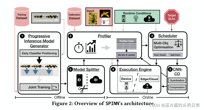
SPINN comprises offline components, run once before deployment, and online components, which operate at run time. Figure 2 shows a high-level view of SPINN. Before deployment,SPINN obtains a CNN model and derives a progressive inference network. This is accomplished by introducing early exits along its architecture and jointly training them using the supplied training set (Section 3.2.1 ). Next, the model splitter component (Section 3.3 2 ) identifies all candidate points in the model where computation can be split between device and cloud. Subsequently, the offline profiler (Section 3.4 3 ) calculates the exit-rate behaviour of the generated progressive model as well as the accuracy of each classifier. Moreover, it measures its performance on the client and server, serving as initial inference latency estimates.
SPINN包含离线部分,在配置之前运行一次,还包含在线部分,在运行时间运行。图2显示了SPINN的高级视图,SPINN获取一个CNN模型并且推导出一个渐进推理网络。 这是通过沿着其结构引入早期出口并且使用提供的训练集联合起来训练它们来实现的(见3.2.1)。此外,模型分割器组件(见3.3.2)识别模型中所有可以在设备和边缘之间划分的候选点。随后,离线分析器计算生成的渐进模型的退出率行为以及每个分类器的准确性。而且,它度量它在客户机和服务器上的性能,作为初始推断延迟估计。
At run time, the scheduler (Section 3.5 4 ) obtains these initial timings along with the target SLAs and run-time conditions and decides on the optimal split and early-exit policy. Given a split point, the communication optimiser (Section 3.6 5 ) exploits the CNN’s sparsity and resilience to reduced bitwidth to compress the data transfer and increase the bandwidth utilisation. The execution engine (Section 3.7 6 ) then orchestrates the distributed inference execution, handling all communication between partitions. Simultaneously, the online profiler monitors the execution across inferences, as well as the contextual factors (e.g. network, device/server load) and updates the initial latency estimates. This way, the system can adapt to the rapidly changing environment, reconfigure its execution and maintain the same QoE.
在运行时间,调度器(见3.5.4)获得这些初始时间以及目标SLAs以及运行时条件,以此决定最优分割和早期退出策略。给定一个分割点,通信优化器(3.6.5)利用CNN的稀疏性和弹性来减少位宽,以压缩数据传输和就增加带宽利用率。然后执行引擎(3.7.6)协调分布式推理的执行,处理分区之间的所有通信。同时,在线分析器监视跨推理的执行以及其他要素(网络,设备/服务器负载)。通过这种方式,系统可以适应快速变化的环境,重新配置其执行并维持相同的QoE.
3.2 渐进推理模型生成器
Given a CNN model, SPINN derives a progressive inference network (Figure 2.1 ). This process comprises a number of key design decisions: 1) the number, position and architecture of intermediate classifiers (early exits), 2) the training scheme and 3) the early-exit policy.
给定一个CNN模型,SPINN生成一个渐进推理模型(图2.1)。这个过程包括许多关键设计决策:1)中间分类器(提前点)的数量,位置和结构、2)训练方案、3)提前退出策略
Early Exits. We place the intermediate classifiers along the depth of the architecture with equal distance in terms of FLOP count. With this platform-agnostic positioning strategy, we are
able to obtain a progressive inference model that supports a wide range of latency budgets while being portable across devices. With respect to their number, we introduce six early exits in order to guarantee their convergence when trained jointly [35, 48], placed at 15%, 30%, . . . 90% of the network’s total FLOPs. Last, we treat the architecture of the early exits as an invariant, adopting the design of [23], so that all exits have the same expressivity [59].
早期退出。我们将中间分类器以相同的FLOP计数方式沿着结构的深度放置。通过这种与平台无关的放置策略,我们能够获得一个渐进的推理模型,该模型支持广泛的延迟预算,同时可以跨设备移植。关于它们的数量,我们引入了6个早期出口,以保证它们在联合训练时的收敛[35,48],放置在15%,30%,…90%的网络总FLOPs中。最后,我们将早期出口的体系结构视为不变式,采用[23]的设计,以便所有出口都具有相同的表达性[59]。
FLOPS(即“每秒浮点运算次数”,“每秒峰值速度”)“每秒所执行的浮点运算次数”(floating-point operations per second)的缩写。因为FLOPS字尾的那个S,代表秒,而不是复数,所以不能省略掉。
Training Scheme. We jointly train all classifiers from scratch and employ the cost function introduced in [35] as follows:


训练方案。我们从头开始联合训练了所有分类器,并且配置了如[35]介绍的成本函数:


Early-exit Policy. For the early-exit strategy, we estimate a classifier’s confidence for a given input using the top-1 output value of its softmax layer (Eq. (1)) [13]. An input takes the i-th exit if the prediction confidence is higher than a tunable threshold, 


提前退出策略。对于提前退出策略,我们使用其softmax层的top-1输出值(Eq.(1))[13]来估计给定输入的分类器的置信度。如果预测置信度高于可调阈值 


Impact of Confidence Threshold.Figure 3 and 4 illustrate the impact of different early-exit policies on the accuracy and early-exit rate of progressive models, by varying the confidence threshold ( 
置信阈值的影响。图3和图4通过改变置信度阈值( 
Based on the figures, we draw two major conclusions that guide the design of SPINN’s scheduler. First, across all networks, we observe a monotonous trend with higher thresholds leading to higher accuracies (Figure 3) while lower ones lead to more samples exiting earlier (Figure 4). This exposes the confidence threshold as a tunable parameter to control accuracy and overall processing time. Second, different networks behave differently, producing confident
predictions at different exits along the architecture. For example, Inception-v3 on CIFAR-100 can obtain a confident prediction earlier on, whereas ResNet-50 on ImageNet cannot classify robustly from early features only. In this respect, we conclude that optimising the confidence threshold for each CNN explicitly is key for tailoring the deployment to the target requirements.
根据这些图,我们得出了指导SPINN调度器设计的两个主要结论。首先,在所有网络中,我们发现一个共有的趋势就是,随着阈值越高精度也越高(图3),而阈值越低则越早退出(图4)。这表示置信度阈值可以作为可调参数来控制精确度和总处理时间。第二,不同的网络行为不同,在架构的不同出口处产生可信预测。比如,CIFAR-100上的Inception-v3能够在早期获得一个可信的预测,而 ImageNet 上的ResNet-50不能仅从早期特征进行稳健分类。在这方面,我们得出结论,明确地优化每个CNN的置信阈值是根据目标需求定制部署的关键。
3.3 模型分割器
After deriving a progressive model from the original CNN, SPINN aims to split its execution across a client and a server in order to dynamically utilise remote resources as required by the application SLAs. The model splitter (Figure 2.2 ) is responsible for 1) defining the potential split points and 2) identifying them automatically in the given CNN.
从原始CNN中得到渐进模型之后,SPINN的目标是在客户机和服务器之间分割它的执行,以便根据应用程序SLAs的要求动态地利用远程资源。模型分割器(图2)负责1)定义潜在的分割点、2)在给定的CNN上自动识别那些被定义过的潜在的分割点。
Split Point Decision Space. CNNs typically consist of a sequence of layers, organised in a feed-forward topology. SPINN adopts a partition scheme which allows splitting the model along its depth at layer granularity. For a CNN with 


分割点决策空间:CNN 通常由一系列层组成,按前馈拓扑组织。SPINN采用一种划分方案,它允许在层粒度上沿着模型的深度分割模型。对于带有 


Automatic Split Point Identification. To automatically detect all candidate split points in the given CNN, the model splitter employs a dynamic analysis approach. This is performed by first constructing the execution graph of the model in the target framework (e.g. PyTorch), identifying all split points and the associated dependencies, and then applying SPINN’s partitioning scheme to yield the final pruned split point space. The resulting set of points defines the allowed partitions that can be selected by the scheduler (Section 3.5).
自动分裂点识别。为了自动检测给定CNN中的所有候选划分点,模型划分器采用了动态分析方法。这是通过首先在目标框架(如PyTorch)中构建模型的执行图,识别所有分裂点和相关依赖,然后应用SPINN的分区方案来生成最终修剪的分割点空间来实现的。结果点集定义了调度程序可以选择的允许分区(第3.5节)。
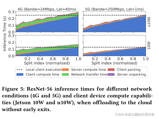
Impact of Split Point. To investigate how the split point selection affects the overall latency, we run multiple CNN splits between a Nvidia Jetson Xavier client and a server (experimental setup detailed in Section 4). Figure 5 shows the breakdown of ResNet-56’s inference times with CIFAR-100 over distinct network conditions and client compute capabilities - u10W and 10W. Packing refers to the runtime of the communication optimiser module, detailed in Section 3.6.
分裂点的影响。为了研究分裂点的选择如何影响整体延迟,我们在Nvidia Jetson Xavier客户端和服务器之间运行多个CNN分支(实验设置详见第4节)。图5显示了在不同的网络条件和客户端计算能力(u10W和10W)下,使用CIFAR-100的ResNet-56推断时间的分解。打包指的是通信优化器模块的运行时间,详细内容见第3.6节。
Based on the figure, we make two observations. First, different split points yield varying trade-offs in client, server and transfer time. For example, earlier splits execute more on the server, while later ones execute more on-device but often with smaller transfer requirements4. This indicates that SPINN’s scheduler can selectively choose one to minimise any given runtime (e.g. device, server or transfer), as required by the user. Second, dynamic conditions such as the connectivity, and the device compute capabilities play an important role in shaping the split point latency characteristics illustrated in Figure 5. For example, a lower-end client (u10W) or a loaded server would require longer to execute its allocated split, while low bandwidth can increase the transfer time. This indicates that it is hard to statically identify the best split point and highlights the need for an informed partitioning that adapts to the environmental conditions in order to meet the application-level performance requirements.
根据这个图,我们做两个观察。首先,不同的分割点会在客户端、服务器和传输时间上产生不同的权衡。例如,早期的分割更多地在服务器上执行,而后期的分割更多地在设备上执行,但通常传输要求更小。这表明SPINN的调度器可以根据用户的要求有选择地选择一个来最小化任何给定的运行时间(例如设备、服务器或传输)。其次,动态条件(如连接性)和设备计算能力在形成图5中所示的分裂点延迟特征方面起着重要作用。例如,低端客户端(u10W)或加载的服务器将需要更长的时间来执行其分配的分割,而低带宽可能会增加传输时间。这表明很难静态地确定最佳分割点,并强调了为了满足应用程序级性能需求,需要适应环境条件的知情分区。
3.4 分析器
Given the varying trade-offs of different split points and confidence thresholds, SPINN considers the client and server load, the networking conditions and the expected accuracy in order to select the most suitable configuration. To estimate this set of parameters, the profiler (Figure 2 ) operates in two stages: i) offline and ii) run-time.
考虑到不同划分点和置信阈值的不同权衡,SPINN考虑客户端和服务器负载、网络条件和预期精度,以选择最合适的配置。为了估计这组参数,分析器(图2)分为两个阶段进行操作:i)离线和ii)运行时
Offline stage: In the offline phase, the profiler performs two kinds of measurements, device-independent and device-specific. The former include CNN-specific metrics, such as 1) the size of data to be transmitted for each candidate split and 2) the average accuracy of the progressive CNN for different confidence thresholds. These are measured only once prior to deployment. Next, the profiler needs to obtain latencies estimates that are specific to each device. To this end, the profiler measures the average execution time perlayer by passing the CNN through a calibration set – sampled from the validation set of the target task. The results serve as the initial
latency and throughput estimates.
脱机阶段:在脱机阶段,分析器执行两种类型的测量,设备独立的和设备特定的。前者包括CNN特定的指标,如1)每个候选分割所传输的数据大小,2)在不同置信阈值下的渐进式CNN的平均准确率。在部署之前,这些度量只进行一次。接下来,分析器需要获取特定于每个设备的延迟估计值。为此,分析器通过将CNN通过从目标任务的验证集取样的校准集来测量每层的平均执行时间,结果作为初始延迟和吞吐量估计。
Run-time stage: At run time, the profiler refines its offline estimates by regularly monitoring the device and server load, as well as the connectivity conditions. To keep the profiler lightweight,
instead of adopting a more accurate but prohibitively expensive estimator, we employ a 2-staged linear model to estimate the inference latency on-device.
运行时阶段:在运行时,分析器通过定期监视设备和服务器负载以及连接条件来改进其离线估计。为了保持分析器的轻量级,我们使用了一个两阶段线性模型来估计设备上的推断延迟,而不是采用一个更准确但昂贵的估计器。
In the first step, the profiler measures the actual on-device execution time up to the split point s, denoted by 

the latency of a different split 

第一步,分析器测量到分割点


Similarly, to assess the server load, the remote end point’s compute latency is optionally communicated back to the device, piggybacked with the CNN response when offloading. If the server does not communicate back latencies for preserving the privacy of the provider, these can be coarsely estimated as . where


类似地,为了评估服务器负载,远程端点的计算延迟可选地通信回设备,在卸载时由CNN响应承载。如果服务器不反馈延迟以保护提供者的隐私,可以粗略地估计为 , 这里,


To estimate the instantaneous network transfer latency, the profiler employs a run-time monitoring mechanism of the bandwidth B and latency L experienced by the device [15]. The overall transfer time is , where


为了估计网络传输的瞬时延迟,分析器采用了运行时监控机制,对设备[15]所经历的带宽B和延迟L进行监控。总体传输时间是,其中


3.5 动态调度器
Given the output of the profiler, the dynamic scheduler (Figure 2) is responsible for distributing the computation between device and cloud, and deciding the early-exit policy of the progressive inference network. Its goal is to yield the highest performing configuration that satisfies the app requirements. To enable the support of realistic multi-criteria SLAs, the scheduler incorporates a combination of hard constraints (e.g. a strict inference latency deadline of 100 ms) and soft targets (e.g. minimise cost on the device side). Internally, we capture these under a multi-objective optimisation (MOO) formulation. The current set of metrics is defined as 


根据分析器的输出,动态调度器(图2)负责在设备和云之间分配计算,并决定渐进推理网络的提前退出策略。它的目标是生成满足应用程序要求的最高性能配置。为了支持现实的多标准SLAs,调度器结合了硬约束(例如100毫秒的严格推断延迟期限)和软目标(例如在设备端最小化成本)。在内部,我们通过多目标优化(MOO)公式捕获这些。当前的度量被定义为


With respect to soft optimisation targets, we define them formally as 

where σ represents a design point, 

关于软优化目标,我们正式将其定义为

其中σ表示设计点

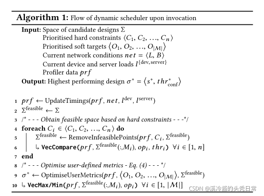
Algorithm 1 presents the scheduler’s processing flow. As a first step, the scheduler uses the estimated network latency and bandwidth, and device and server loads to update the profiler parameters (line 1), including the attainable latency and throughput, and device and server cost for each candidate configuration. Next, all infeasible solutions are discarded based on the supplied hard constraints (lines 4-7); given an ordered tuple of prioritised constraints


算法1给出了调度程序的处理流程。作为第一步,调度器使用估计的网络延迟和带宽,以及设备和服务器负载来更新分析器参数(第1行),包括可达到的延迟和吞吐量,以及每个候选配置的设备和服务器成本。接下来,根据所提供的硬约束丢弃所有不可行的解(第4-7行);给定一个有序元组的优先约束


Deployment. Upon deployment, the scheduler is run on the client side, since most relevant information resides on-device. In a multi-client setting, this setup is further reinforced by the fact that each client device decides independently on its offloading parameters. However, to be deployable without throttling the resources of the target mobile platform, the scheduler has to yield low resource utilisation at run time. To this end, we vectorise the comparison, maximisation and minimisation operations (lines 5-6 and 9-10 in Algorithm 1) to utilise the SIMD instructions of the target mobile CPU (e.g. the NEON instructions on ARM-based cores) and minimise the scheduler’s runtime.
部署。在部署时,调度器在客户端运行,因为大多数相关信息驻留在设备上。在多客户端设置中,每个客户端设备独立地决定其卸载参数,这一事实进一步加强了这种设置。然而,要在不限制目标移动平台资源的情况下进行部署,调度器必须在运行时产生较低的资源利用率。为此,我们对比较、最大化和最小化操作(算法1中的第5-6行和第9-10行)进行矢量化,以利用目标移动CPU的SIMD指令(例如基于arm的内核上的NEON指令),并最小化调度程序的运行时间。
At run time, although the overhead of the scheduler is relatively low, SPINN only reevaluates the candidate configurations when the outputs of the profiler change by more than a predefined threshold. For highly transient workloads, we can switch from a moving average to an exponential back-off threshold model for mitigating too many scheduler calls. The scheduler overhead and the tuning of the invocation frequency is discussed in Section 4.3.2.
在运行时,尽管调度器的开销相对较低,但只有当分析器的输出更改超过预定义的阈值时,SPINN才会重新评估候选配置。对于特别短暂的工作负载,我们可以从移动平均值切换到指数后退阈值模型,以减少过多的调度器调用。调度器开销和调用频率的调优将在第4.3.2节中讨论。
The server – or HA proxy5[70] in multi-server architectures –can admit and schedule requests on the remote side to balance the workload and minimise inference latency, maximise throughput or minimise the overall cost by dynamically scaling down unused resources. We consider these optimisations cloud-specific and out of the scope of this paper. As a result, in our experiments we account for a single server always spinning and having the model resident to its memory. Nevertheless, in a typical deployment, we would envision a caching proxy serving the models with RDMA to the CPU or GPU of the end server, in a virtualised or serverless environment so as to tackle the cold-start problem [57, 77]. Furthermore, to avoid oscillations (flapping) of computation between the deployed devices and the available servers, techniques used for data-center traffic flapping are employed [5].
3.6 CNN通信优化器
CNN layers often produce large volumes of intermediate data which come with a high penalty in terms of network transfer. A key enabler in alleviating the communication bottleneck in SPINN is the communication optimiser module (CNN-CO) (Figure 2 ). CNN-CO comprises two stages. In the first stage, we exploit the resilience of CNNs to low-precision representation [14, 16, 28, 38] and lower the data precision from 32-bit floating-point down to 8-bit fixed-point through linear quantisation [28, 53]. By reducing the bitwidth of only the data to be transferred, our scheme allows the transfer size to be substantially lower without significant impact on the accuracy of the subsequent classifiers (i.e. <0.65 percentage point drop across all exits of the examined CNNs). Our scheme differs from both i) weights-only reduction [17, 67, 86], which minimises the model size rather than activations’ size and ii) all-layers quantisation [14, 16,24, 28] which requires complex techniques, such as quantisation- aware training [24, 28] or a re-training step [14, 16], to recover the accuracy drop due to the precision reduction across all layers.
CNN层经常产生大量的中间数据,这在网络传输方面带来了很高的代价。缓解SPINN中通信瓶颈的一个关键使能器是通信优化器模块(CNN-CO)(图2 5)。CNN-CO包括两个阶段。在第一阶段,我们利用cnn对低精度表示的弹性[14,16,28,38],并通过线性量化将数据精度从32位浮点数降低到8位定点[28,53]。通过仅减少要传输的数据的位宽,我们的方案允许传输大小大大降低,而不会对后续分类器的准确性产生重大影响(即在经过检查的cnn的所有出口下降<0.65个百分点)。我们的方案与以下两种方案不同:i)只减重[17,67,86],它最小化了模型大小,而不是激活的大小;ii)全层量化[14,16,24,28],它需要复杂的技术,如量化感知训练[24,28]或再训练步骤[14,16],恢复所有层精度降低造成的精度下降。
The second stage exploits the observation that activation data are amenable to compression. A significant fraction of activations are zero-valued, meaning that they are sparse and highly com- pressible. As noted by prior works [56, 60, 82], this sparsity of activations is due to the extensive use of the ReLU layer that follows the majority of layers in modern CNNs. In CNN-CO, sparsity is further magnified due to the reduced precision. In this respect, CNN-CO leverages the sparsity of the 8-bit data by means of an LZ4 compressor with bit shuffling.
第二阶段利用活化数据易于压缩的观察结果。很大一部分激活是零值的,这意味着它们是稀疏的和高度可压缩的。正如之前的工作[56,60,82]所指出的,这种激活的稀疏性是由于广泛使用了ReLU层,而ReLU层在现代cnn的大多数层之后。在CNN-CO中,由于精度降低,稀疏性进一步放大。在这方面,CNN-CO通过带有位变换的LZ4压缩器利用8位数据的稀疏性。
At run time, SPINN predicts whether the compression cost will outweigh its benefits by comparing the estimated CNN-CO runtime to the transfer time savings. If CNN-CO’s overhead is amortised, SPINN queues offloading requests’ data to the CNN-CO, with dedicated threads for each of the two stages, before transmission. Upon reception at the remote end, the data are decompressed and cast back to the original precision to continue inference. The overhead is shown as packing in Figure 5 for non-progressive models.
在运行时,SPINN通过比较估计的CNN-CO运行时和节省的传输时间来预测压缩成本是否会超过它的好处。如果CNN-CO的开销被分摊,那么在传输之前,SPINN队列将请求的数据卸载到CNN-CO,每个阶段都有专门的线程。在远端接收到数据后,数据被解压缩并转换回原来的精度以继续推断。开销如图5中为非渐进式模型所示。
3.7 分布式执行引擎
In popular Deep Learning frameworks, such as TensorFlow [1] and PyTorch [58], layers are represented bymodules and data in the form of multi-dimensional matrices, called tensors. To split and offload computation, SPINN modifies CNN layer’s operations behind the scenes. To achieve this, it intercepts module and tensor operations by replacing their functions with a custom wrapper using Python’s function decorators.
在流行的深度学习框架中,如TensorFlow[1]和PyTorch[58],层是由称为张量的多维矩阵形式的模块和数据表示的。为了拆分和卸载计算,SPINN在后台修改了CNN层的操作。为了实现这一点,它通过使用Python的函数装饰器将模块和张量操作替换为自定义包装器的函数来拦截它们。
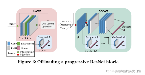
Figure 6 focuses on an instance of an example ResNet block. SPINN attributes IDs to each layer in a trace-based manner, by executing the network and using the layer’s execution order as a sequence identifier.6SPINN uses these IDs to build an execution graph in the form of a directed acyclic graph (DAG), with nodes representing tensor operations and edges the tensor flows among them [1, 62, 75]. This is then used to detect the dependencies acrosspartitions. To achieve this, Python’s dynamic instance attribute registration is used totainttensors and monitor their flow through the network. With Figure 6 as a reference, SPINN’s custom wrapper (Figure 2 6 ) performs the following operations:
图6重点介绍了一个示例ResNet块的实例。通过执行网络并使用层的执行顺序作为序列标识符,SPINN以基于跟踪的方式为每一层添加属性id。SPINN使用这些id构建一个有向无环图(DAG)形式的执行图,其中节点表示张量操作,边表示张量在其中流动[1,62,75]。然后用它来检测跨分区的依赖关系。为了实现这一点,Python的动态实例属性注册被用于控制张量,并通过网络监控它们的流。参考图6,SPINN的自定义包装器(图2)执行以下操作:
Normal execution: When a layer is to be run locally, the wrap- per calls the original function it replaced. In Figure 6, layers 1 to 8 execute normally on-device, while layers from 9 until the end
execute normally on the server side.
正常执行:当一个层要在本地运行时,包装器调用它所替换的原始函数。在图6中,第1层到第8层在设备上正常执行,而第9层到最后一层在服务器端正常执行。
Offload execution:When a layer is selected as a partition point (layer 9), instead of executing the original computation on the client, the wrapper queues an offloading request to be transmitted. This request contains the inputs (layer 5’s output) and subsequent layer dependencies (input of skip connection). Furthermore, the inference and the data transfer are decoupled in two separate threads, to allow for pipelining of data transfer and next frame processing.
卸载执行:当选择一个层作为分区点(第9层)时,包装器不是在客户机上执行原始计算,而是将要传输的卸载请求排队。这个请求包含输入(第5层的输出)和随后的层依赖(跳过连接的输入)。此外,推理和数据传输在两个独立的线程中解耦,以允许数据传输和下一帧处理的流水线操作。
Resume execution: Upon receiving an offloading request, the inputs and dependencies are injected in the respective layers (layer 9 and add operation) and normal execution is resumed on the remote side. When the server concludes execution, the results are sent back in a parallel thread.
恢复执行:在接收到卸载请求时,将输入和依赖项注入到各自的层中(第9层和add操作),并在远程端恢复正常执行。当服务器结束执行时,结果将在一个并行线程中发送回来。
Early exit:When an intermediate classifier (i.e.early exit) is exe- cuted, the wrapper evaluates its prediction confidence (Eq. (1)). If it is above the providedthrconf, execution terminates early, returning the current prediction (Eq. (2)).
早期退出:当一个中间分类器(即早期退出)被执行时,包装器计算它的预测置信度(Eq.(1))。如果它高于providdthrconf,则执行提前终止,返回当前预测(Eq.(2))。
Since the premise of our system is to always have at least one usable result on the client side, we continue the computation on-device even past the split layer, until the next early exit is encountered. Furthermore, to avoid wasteful data transmission and redundant computation, if a client-side early exit covers the latency SLA and satisfies the selected thrconf, the client sends a termination signal to the remote worker to cancel the rest of the inference. If remote execution has not started yet, SPINN does not offload at all.
由于我们的系统的前提是在客户端总是有至少一个可用的结果,所以我们继续在设备上进行计算,甚至超过了分裂层,直到遇到下一个早期出口。此外,为了避免浪费的数据传输和冗余计算,如果客户端早期退出覆盖了延迟SLA并满足选定的thrconf,客户端向远程工作者发送终止信号以取消推断的其余部分。如果远程执行尚未开始,则SPINN根本不会卸载。
四、评估
This section presents the effectiveness of SPINN in significantly improving the performance of mobile CNN inference by examining its core components and comparing with the currently standard device-and cloud-only implementations and state-of-the-art collaborative inference systems.
本节通过检查SPINN的核心组件,并与当前的标准设备和仅云实现以及最先进的协作推理系统进行比较,展示SPINN在显著提高移动CNN推理性能方面的有效性。
4.1 实验装置
For our experiments, we used a powerful computer as the server and an Nvidia Jetson Xavier AGX as the client (Table 1). Specifically for Jetson, we tested against three different power profiles to emulate end-devices with different compute capabilities1) 30W (full power), 2) 10W (low power), 3) underclocked 10W (u10W). Furthermore, to study the effect of limited computation capacity (e.g. high-load server), we emulated the load by linearly scaling up the CNN computation times on the server side. We simulated the network conditions of offloading by using the average bandwidth and latency across national carriers [26, 27], for 3G, 4G and 5G mobile networks. For local-area connections (Gigabit Ethernet 802.3, WiFi-5 802.11ac), we used the nominal speeds of the protocol. We have developed SPINN on top of PyTorch (1.1.0) and experimented with four models, altered from torchvision (0.3.0) to include early exits or to reflect the CIFAR-specific architectural changes. We evaluated SPINNusing: ResNet-50 and -56 [20], VGG16 [63], MobileNetV2 [61] and Inception-v3 [69]. Unless stated otherwise, each benchmark was run 50 times to obtain the average latency.
在我们的实验中,我们使用一个强大的计算机作为服务器和一个Nvidia Jetson Xavier AGX作为客户机(表1),专门为Jetson,我们测试了对三个不同的权力配置文件来模拟终端设备与不同的计算能力:1)30 w(全功率),2)10 w(低功率),3)underclocked 10 w (u10W)。此外,为了研究有限计算能力(例如高负载服务器)的影响,我们通过在服务器端线性增加CNN计算时间来模拟负载。我们利用全国各运营商的平均带宽和延迟[26,27],模拟3G、4G和5G移动网络卸载的网络条件。对于本地连接(Gigabit Ethernet 802.3, WiFi5 802.11ac),我们使用协议的名义速度。我们在PyTorch(1.1.0)的基础上开发了SPINN,并尝试了四种模型,从torchvision(0.3.0)改变为包括早期出口或反映ci远远地架构变化。我们评估了SPINNusing: ResNet-50和-56 [20],VGG16 [63], MobileNetV2[61]和incepsion -v3[69]。除非另有说明,否则每个基准测试都会运行50次以获得平均延迟。
Datasets and Training. We evaluated SPINN on two datasets, namely CIFAR-100 [41] and ImageNet (ILSVRC2012) [10]. The former contains 50k training and 10k test images of resolution 32×32,each corresponding to one of 100 labels. The latter is significantly larger, with 1.2m training and 50k test images of 300×300 and 1000 labels. We used the preprocessing steps described in each model’s implementation, such as scaling and cropping the input image, stochastic image flip (p = 0.5) and colour channel normalisation. After converting these models to progressive early-exit networks, we trained them jointly from scratch end-to-end, with the “overthink" cost function (Section 3.2). We used the authors’ training hyperparameters, except for MobileNetV2, where we utilised SGD with learning rate of 0.05 and cosine learning rate scheduling, due to convergence issues. We trained the networks for 300 epochs on CIFAR-100 and 90 epochs on ImageNet.
数据集和训练。我们在两个数据集上评估SPINN,即CIFAR-100[41]和ImageNet (ILSVRC2012)[10]。前者包含50k训练图像和10k测试图像,分辨率为32×32,分别对应100个标签中的一个。后者要大得多,有120万训练图像和50万测试图像300×300和1000个标签。我们使用了每个模型实现中描述的预处理步骤,如缩放和裁剪输入图像,随机图像翻转(p = 0.5)和彩色通道归一化。在将这些模型转换为渐进的早期退出网络之后,我们使用“过度思考”成本函数(第3.2节),从零开始对它们进行联合训练。我们使用了作者的训练超参数,除了MobileNetV2,其中由于收敛问题,我们使用学习率为0.05的SGD和余弦学习率调度。我们在CIFAR-100上训练了300个epoch,在ImageNet上训练了90个epoch。
4.2 性能比较
This subsection presents a performance comparison of SPINN with:1) the two state-of-the-art CNN offloading systems Neurosurgeon[34] andEdgent[46] (Section 2); 2) the status-quo cloud- and device-only baselines; and 3) a non-progressive ablated variant of SPINN.
本小节介绍了spin与以下两种系统的性能比较:1)两种最先进的CNN卸载系统Neurosurgeon[34]和dedgent [46] (Section 2);2)仅云和设备基线的现状;3) SPINN的非渐进式烧蚀变体。
4.2.1 Throughput Maximisation. Here, we assessSPINN’s inference throughput across varying network conditions. For these experi- ments, the SPINN schedulerâĂŹs objectives were set to maximise throughput with up to 1 percentagepoint (pp)tolerance in accuracy drop with respect to the CNN’s last exit.
4.2.1吞吐量最大化。准备这里,我们评估了spinn在不同网络条件下的推理吞吐量。对于这些实验,SPINN schedulerâĂŹs的目标被设置为最大吞吐率,与CNN的最后一次退出相比,准确率下降高达1个百分点(pp)的公差。
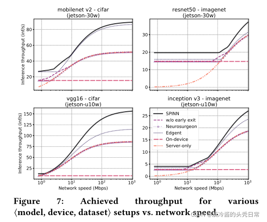
Figure 7 shows the achieved inference throughput for varying network speeds. On-device execution yields the same throughput independently of the network variation, but is constrained by the processing power of the client device. Server-only execution follows the trajectory of the available bandwidth. Edgent always executes a part of the CNN (up to the exit that satisfies the 1pp accuracy tolerance) irrespective of the network conditions. As a result, it follows a similar trajectory to server-only but achieves higher throughput due to executing only part of the model. Neurosurgeon demonstrates a more polarised behaviour; under constrained connectivity it executes the whole model on-device, whereas as bandwidth increases it switches to offloading all computation as it results in higher throughput. The ablated variant of SPINN (i.e. without early exits) largely follows the behaviour of Neurosurgeon at the two extremes of the bandwidth while in the middle range, it is able to achieve higher throughput by offloading earlier due to CNN-CO compressing the transferred data.
图7显示了在不同网络速度下实现的推理吞吐量。设备上执行产生独立于网络变化的相同吞吐量,但受到客户端设备处理能力的限制。仅服务器执行遵循可用带宽的轨迹。无论网络条件如何,Edgent总是执行CNN的一部分(直到满足1pp精度公差的出口)。因此,它遵循类似于只执行服务器的轨迹,但由于只执行模型的一部分而实现更高的吞吐量。神经外科医生表现出更两极分化的行为;在有限的连接性下,它在设备上执行整个模型,而随着带宽的增加,它切换到卸载所有的计算,因为它导致更高的吞吐量。在带宽的两个极端,烧断的SPINN变体(即没有早期退出)在很大程度上遵循神经外科医生的行为,而在中间范围,由于CNN-CO压缩传输数据,它能够通过提前卸载实现更高的吞吐量。
The end-to-end performance achieved by SPINN delivers the highest throughput across all setups, achieving a speedup of up to 83% and 52% over Neurosurgeon and Edgent, respectively. This can be attributed to our bandwidth- and data-locality-aware scheduler choices on the early-exit policy and partition point. In low bandwidths,SPINNselects device-only execution, outperforming all other on-device designs due to its early-exiting mechanism, tuned by the scheduler module. In the mid-range, the CNN-CO module enables SPINN to better utilise the available bandwidth and start offloading earlier on, outperforming both Edgent and Neurosurgeon. In high-bandwidth settings, our system surpasses the performance of all other designs by exploiting its optimised early-exiting scheme.
SPINN实现的端到端性能在所有设置中提供了最高的吞吐量,比Neurosurgeon和Edgent分别实现了高达83%和52%的加速。这可以归因于我们在早期退出策略和分区点上选择了支持带宽和数据位置的调度器。在低带宽中,spinnselect设备执行,由于其早期退出机制,优于所有其他设备上的设计,由调度器模块进行调优。在中端,CNN-CO模块使SPINN能够更好地利用可用带宽,并更早开始负载,优于Edgent和Neurosurgeon。在高带宽设置中,我们的系统通过利用其优化的早期退出方案,超越了所有其他设计的性能。
Specifically, compared to Edgent, SPINN takes advantage of the input’s classification difficulty to exit early, whereas the latter only selects an intermediate exit to uniformly classify all incoming samples. Moreover, in contrast with Edgent’s strategy to always transmit the input to the remote endpoint, we exploit the fact that data already reside on the device and avoid the wasteful data transfers.
具体来说,与Edgent相比,SPINN利用输入的分类难度提前退出,而后者只选择一个中间退出,对所有进入的样本进行统一分类。此外,与Edgent总是将输入传输到远程端点的策略不同,我们利用了数据已经驻留在设备上的事实,避免了浪费的数据传输。
4.2.2 Server-Load Variation. To investigate the performance of SPINN under various server-side loads, we measured the inference throughput of SPINN against baselines when varying the load of the remote end, with 1pp of accuracy drop tolerance. This is accomplished by linearly scaling the latency of the server execution by a slowdown factor (i.e. a factor of 2 means the server is 2× slower). Figure 8 presents the throughput achieved by each approach under various server-side loads, with the Jetson configured at the 10W profile and the network speed in the WiFi-5 range (500 Mbps).
4.2.2服务器负载变化。为了研究SPINN在不同服务器端负载下的性能,我们测量了在改变远程端负载时SPINN的推理吞吐量与基线的关系,精度下降容忍度为1pp。这是通过将服务器执行的延迟线性扩展到一个减速因子(即,2的系数意味着服务器的速度是2倍)来实现的。图8展示了在各种服务器端负载下每种方法实现的吞吐量,其中Jetson配置为10W配置文件,网络速度在WiFi-5范围内(500 Mbps)。
With low server load (left of the x-axis), the examined systems demonstrate a similar trend to the high-bandwidth performance of Figure 7. As the server becomes more loaded (i.e. towards the right-hand side), performance deteriorates, except for the case of device-only execution which is invariant to the server load. On the one hand, although its attainable throughput reduces, Neurosurgeon adapts its policy based on the server utilisation and gradually executes a greater fraction of the CNN on the client side. On the other hand, Edgent’s throughput deteriorates more rapidly and even reaches below the device-only execution under high server load, since its run-time mechanism does not consider the varying server load. Instead, by adaptively optimising both the split point and the early-exit policy, SPINN’s scheduler manages to adapt the overall execution based on the server-side load, leading to throughput gains between 1.18-1.99× (1.57× geo. mean) and 1.15-3.09× (1.61× geo. mean) over Neurosurgeon and Edgent respectively.
在服务器负载较低的情况下(x轴左侧),所检查的系统显示了与图7所示的高带宽性能类似的趋势。当服务器负载增加(即向右侧)时,性能就会下降,除了设备执行的情况,这对服务器负载是不变的。一方面,尽管其可达到的吞吐量降低了,但神经外科医生根据服务器利用率调整其策略,并逐渐在客户端执行更大比例的CNN。另一方面,由于其运行时机制不考虑不断变化的服务器负载,Edgent的吞吐量恶化得更快,甚至在高服务器负载下达到仅设备执行的水平。相反,通过自适应地优化分裂点和提前退出策略,SPINN的调度器设法根据服务器端负载调整整体执行,从而获得1.18-1.99× (1.57× geo)之间的吞吐量增益。平均值)和1.15-3.09× (1.61× geo.)平均值)分别超过神经外科和边缘外科。
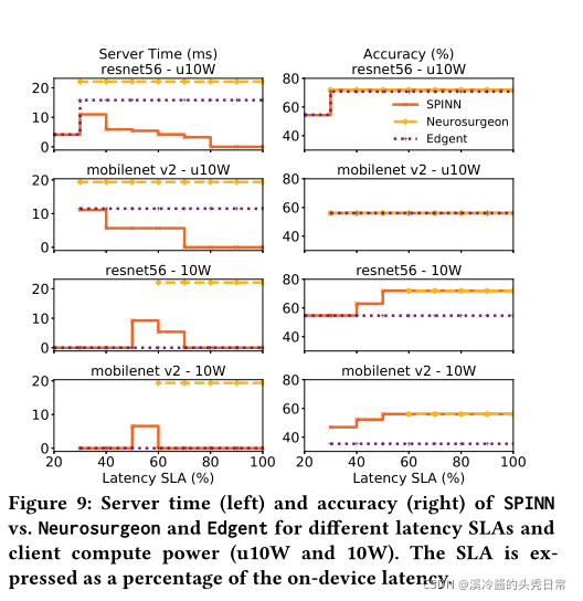
4.2.3 Case Study: Latency-driven SLAs at minimal server cost. To assess SPINN’s performance under deadlines, we target the scenario where a service provider aims to deploy a CNN-based application that meets strict latency SLAs at maximum accuracy and minimal server-side cost. In this setting, we compare againstNeurosurgeon8 and Edgent, targeting MobileNetV2 and ResNet-56 over 4G. Figure 9 shows the server computation time and accuracy achieved by each system for two device profiles with different compute capabilities -u10W and 10W. Latency SLAs are represented as a percentage of the device-only runtime of the original CNN (i.e. 20% SLA means that the target is5×less latency than on-device execution, requiring early exiting and/or server support).
4.2.3案例研究:以最小服务器成本实现延迟驱动的sla。为了在最后期限内评估SPINN的性能,我们的目标是这样一个场景:服务提供商旨在部署一个基于cnn的应用程序,该应用程序以最大的准确性和最小的服务器端成本满足严格的延迟sla。在这种情况下,我们比较了neurosurgeon8和Edgent,目标是4G以上的MobileNetV2和ResNet-56。图9显示了两个具有u10W和10W不同计算能力的设备概要的服务器计算时间和精度。延迟SLA表示为原始CNN的仅设备运行时间的百分比(即20% SLA意味着,目标is5×less的延迟比设备上的执行时间,需要提前退出和/或服务器支持)。
For the low-end device (u10W) and strict latency deadlines, SPINNoffloads as much as possible to the cloud as it allows reaching faster a later exit in the network, hence increasing the accuracy. As the SLA loosens (reaching more than 40% of the on-device latency), SPINN starts to gradually execute more and more locally. In contrast, Edgent and Neurosurgeon achieve similar accuracy but with up to 4.9× and 6.8× higher server load. On average across all targets, SPINN reduces Edgent and Neurosurgeon server times by 68.64% and 82.5% (60.3% and 83.6% geo. mean), respectively, due to its flexible multi-objective scheduler. Instead, Neurosurgeon can only optimise for overall latency and cannot trade off accuracy to meet the deadline (e.g. for 20% SLA on ResNet-56) while Edgent cannot account for server-time minimisation and accuracy drop constraints.
对于低端设备(u10W)和严格的延迟期限,spinnoff尽可能多地加载到云,因为它允许更快地到达网络的更晚出口,从而提高准确性。随着SLA的放松(达到超过40%的设备上延迟),SPINN开始逐渐越来越多地在本地执行。相比之下,Edgent和Neurosurgeon的准确率相似,但服务器负载最高可达4.9×和6.8×。在所有目标上,SPINN平均减少了68.64%和82.5%的Edgent和神经外科医生服务器时间(60.3%和83.6% geo。,由于其灵活的多目标调度。相反,神经外科医生只能优化总体延迟,而不能牺牲准确性来满足截止日期(例如,在ResNet-56上的20% SLA),而edge不能考虑服务器时间最小化和准确性下降的约束。
The situation is different for the more powerful device (10W). With the device being faster, the SLA targets become much stricter. Therefore, we observe that SPINN and Edgent can still meet a latency constraint as low as 20% and 30% of the local execution time for ResNet-56 and MobileNetV2 respectively. In contrast, without progressive inference, it is impossible for Neurosurgeon to achieve inference latency below 60% of on-device execution across both CNNs. In this context, SPINN is able to trade off accuracy in order to meet stricter SLAs, but also improve its attainable accuracy as the latency constraints are relaxed.
对于功率更大的设备(10W),情况有所不同。随着设备的速度加快,SLA目标变得更加严格。因此,我们观察到,对于ResNet-56和MobileNetV2, SPINN和Edgent仍然可以分别满足低至本地执行时间的20%和30%的延迟约束。相比之下,如果没有渐进式推理,神经外科医生不可能在两个cnn上实现低于60%的设备执行推理潜伏期。在这种情况下,SPINN能够权衡精度以满足更严格的sla,但也可以随着延迟约束的放松而提高其可达到的精度。
For looser latency deadlines (target larger than 50% of the on-device latency), SPINN achieves accuracy gains of 17.3% and 20.7% over Edgent for ResNet-56 and MobileNetV2, respectively. The reason behind this is twofold. First, when offloading, Edgent starts the computation on the server side, increasing the communication latency overhead. Instead, SPINN’s client-to-server offloading strategy and compression significantly reduces the communication latency overhead. Second, due to Edgent’s unnormalised cost function ( )the throughput’s reward dominates the accuracy gain, leading to always selecting the first early-exit subnetwork and executing it locally. In contrast, SPINN’s scheduler’s multi-criteria design is able to capture accuracy, server time and latency constraints to yield an optimised deployment. Hence, similarly to the slower device, SPINN successfully exploits the server resources to boost accuracy under latency constraints, while it can reach up to pure on-device execution for loose deadlines.
对于较宽松的延迟期限(目标大于设备上延迟的50%),SPINN在ResNet-56和MobileNetV2上分别实现了17.3%和20.7%的精度增益。这背后的原因是双重的。首先,当卸载时,Edgent在服务器端开始计算,增加了通信延迟开销。相反,SPINN的客户端到服务器的卸载策略和压缩显著降低了通信延迟开销。其次,由于Edgent的非标准化成本函数(),吞吐量的回报支配着精度增益,导致总是选择第一个提前退出的子网并在本地执行它。相比之下,SPINN的调度器的多标准设计能够捕获准确性、服务器时间和延迟约束,从而产生优化的部署。因此,与较慢的设备类似,SPINN成功地利用服务器资源在延迟约束下提高精度,而对于松散的截止日期,它可以达到纯粹的设备上执行。
4.3 运行时开销开销和效率
4.3.1 Deployment Overhead. By evaluating across our examined CNNs and datasets on the CPU of Jetson, the scheduler executes in max 14 ms (11 ms geo. mean). This time includes the cost of reading the profiler parameters, updating the monitored metrics, and searching for and returning the selected configuration. Moreover, SPINN’s memory consumption is in the order of a few KB (i.e.<1% of Jetson’s RAM). These costs are amortised over multiple inferences, as the scheduler is invoked only on significant context changes. We discuss the selection of such parameters in the following section.
4.3.1部署开销。通过在Jetson的CPU上评估我们检查过的cnn和数据集,调度器最多执行14毫秒(11毫秒地理位置)。的意思)。这一次包括读取分析器参数、更新监控指标以及搜索和返回所选配置的成本。此外,SPINN的内存消耗大约是几个KB(即< Jetson的RAM的1%)。这些成本在多个推断上分摊,因为调度程序只在上下文发生重大更改时调用。我们将在下一节讨论这些参数的选择。
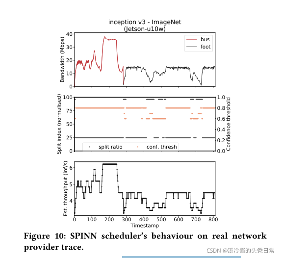
4.3.2 Network Variation. To assess the responsiveness of SPINN in adapting to dynamic network conditions, we targeted a real bandwidth trace from a Belgian ISP. The trace contains time series of network bandwidth variability during different user activities. In this setup, SPINN executes the ImageNet-trained Inception-v3 with Jetson-u10W as the client under the varying bandwidth emulated by the Belgium 4G/LTE logs. The scheduler is configured to maximise both throughput and accuracy. Figure 10 (top) shows an example bandwidth trace from a moving bus followed by walking. Figure 10 (bottom) shows SPINN’s achieved inference throughput under the changing network quality. The associated scheduler decisions are depicted in Figure 10.
4.3.2网络变化。为了评估spin适应动态网络条件的响应性,我们以比利时ISP提供的真实带宽跟踪为目标。跟踪包含了不同用户活动期间网络带宽变化的时间序列。在这个设置中,spin使用Jetson-u10W作为客户端,在比利时4G/LTE日志模拟的可变带宽下执行imagenet训练的inction -v3。调度程序被配置为最大的吞吐量和准确性。图10(顶部)显示了一个示例带宽跟踪,该跟踪来自一辆移动的公共汽车,随后是步行。图10(底部)显示了在网络质量不断变化的情况下,SPINN获得的推理吞吐量。图10(中间)描述了相关的调度器决策。
At low bandwidth (<5 Mbps), SPINN falls back to device-only execution. In these cases, the scheduler adopts a less conservative early-exit policy by lowering the confidence threshold. In this manner, it allows more samples to exit earlier, compensating for the client’s low processing power. Nonetheless, the impact on accuracy remains minimal (<1%) for the selected early-exit policies by the scheduler (thrconf∈ [0.6,1.0]), as illustrated in Figure 3 for Inception-v3 on ImageNet. At the other end, high bandwidths result in selecting an earlier split point and thus achieving up to 7× more inf/sec over pure on-device execution. Finally, the similar trajectories of the top and bottom figure suggest that our scheduler can adapt the system to the running conditions, without having to be continuously invoked.
在低带宽(<5 Mbps)时,SPINN回落到只执行设备。在这些情况下,调度器通过降低置信度阈值,采用不那么保守的提前退出策略。通过这种方式,它允许更多的样本更早地退出,弥补了客户端较低的处理能力。尽管如此,对于调度程序所选择的早期退出策略(thrconf∈[0.6,1.0]),其对准确性的影响仍然是最小的(<1%),如图3中ImageNet上Inception-v3所示。在另一端,高带宽导致选择更早的分裂点,从而达到7×更多inf/sec比纯设备上执行。最后,顶部和底部图的相似轨迹表明,我们的调度程序可以使系统适应运行条件,而无需连续调用。
Overall, we observe that small bandwidth changes do not cause significant alterations to the split and early-exit strategies. By employing an averaging historical window of three values and a difference threshold of 5%, the scheduler is invoked 1/3 of the total bandwidth changes across traces.
总的来说,我们观察到小的带宽变化不会导致分裂和早期退出策略的显著变化。通过使用三个值的平均历史窗口和5%的差异阈值,调度器将在跟踪过程中调用总带宽变化的1/3。
4.4 能量消耗
Figure 11 shows the breakdown of dominant energy consumption across the client device subsystems. We measured energy consumption over 1000 inferences from the validation set and offloading over UK’s Three Broadband’s 4G network with a Huawei E3372 USB adapter. We measured the power of Jetson (CPU, GPU) from its integrated probes and the transmission energy with the Monsoon AAA10F power monitor.
图11显示了跨客户机设备子系统的主要能源消耗的细分。通过华为E3372USB适配器,我们测量了超过1000条来自英国Three Broadband 4G网络验证集和卸载的能耗。我们通过Jetson (CPU, GPU)的集成探头和Monsoon AAA10F功率监视器测量传输能量。
Traversing the horizontal axis left-to-right, we first see device-only execution without and with early-exits, where the local processing dominates the total energy consumption. The latter shows benefits due to samples exiting early from the network. Next, we showcase the consumption breakdown of three different 〈split,thrconf〉 configurations. The first two configurations demonstrate comparable energy consumption with the device-only execution without early exits. On the contrary, a bad configuration requires an excessively large transfer size, leading to large compression and transfer energy overheads. Last, the energy consumption when fully offloading is dominated by the network transfer.
从左到右遍历水平轴,我们首先看到只有设备执行没有早期退出,其中本地处理占总能量消耗的主导地位。后者显示了由于样本提前退出网络而带来的好处。接下来,我们展示三个不同的〈split,thrconf〉配置的消费分解。前两个配置演示了在没有早期退出的情况下仅执行设备的能耗。相反,糟糕的配置需要过大的传输大小,从而导致较大的压缩和传输能量开销。最后,完全卸载时的能耗由网络传输控制。
Across configurations, we witness a 5× difference in energy consumption across different inference setups. While device-only execution yields the lowest energy footprint per sample, it is also the slowest. Our scheduler is able to yield deployments that are significantly more energy efficient than full offloading (4.2×) and on par with on-device execution (0.76 − 1.12×), while delivering significantly faster end-to-end processing. Finally, with different configurations varying both in energy and performance, the decision space is amenable to energy-driven optimisation by adding energy as a scheduler optimisation metric.
在不同的配置中,我们发现不同推理设置的能量消耗有5倍的差异。虽然仅设备执行每个样本产生最低的能量占用,但它也是最慢的。我们的调度器能够提供比完全卸载(4.2×)更节能的部署,与设备上执行(0.76−1.12×)相当,同时提供显著更快的端到端处理。最后,由于不同的配置在能量和性能上都是不同的,决策空间可以通过添加能量作为调度程序的优化指标来接受能量驱动的优化。
4.5 限制可用性鲁棒性
Next we evaluate SPINN’s robustness under constrained availability of the remote end such as network timeouts, disconnections and server failures. More specifically, we investigate 1) the achieved accuracy across various failure rates and 2) the latency improvement over conventional systems enhanced with an error-control policy. In these experiments, we fix the confidence threshold of three models (Inception-v3, ResNet-56 and ResNet-50) to a value of 0.8 and emulate variable failure rates by sampling from a random distribution across the validation set.
接下来,我们评估SPINN在网络超时、断开连接和服务器故障等受限的远程端可用性下的健壮性。更具体地说,我们研究了1)在不同失败率下所实现的准确率,2)与通过错误控制策略增强的传统系统相比,延迟的改善。在这些实验中,我们将三个模型(Inception-v3, ResNet-56和ResNet-50)的置信度阈值固定为0.8,并通过从整个验证集的随机分布中取样来模拟变量失败率。
Accuracy comparison: For this experiment (Figure 12), we compare SPINN at different network split points (solid colours) against a non-progressive baseline (dashed line). Under failure conditions, the baseline unavoidably misclassifies the result as there is no usable result locally on-device. However, SPINN makes it possible to acquire the most confident local result up to the split point, when the server is unavailable.
精度比较:在这个实验中(图12),我们将SPINN在不同的网络分裂点(纯色)与非渐进式基线(虚线)进行比较。在失败条件下,基线不可避免地将结果错误分类,因为在设备本地没有可用的结果。然而,当服务器不可用时,SPINN使得在分裂点之前获得最可靠的本地结果成为可能。
As shown in Figure 12, the baseline quickly drops in accuracy as the failure rate increases. This is not the case with SPINN, whichmanages to maintain a minimal accuracy drop. Specifically, we witness drops ranging in [0,5.75%] for CIFAR-100 and [0.46%,33%] for ImageÎİet, when the equivalent drop of the baseline is[11.56%,44.1%] and [9.25%,44.34%], respectively. As expected, faster devices are able to execute locally a larger part of the model (exit later) while meeting their SLA exhibit the smallest impact under failure, as depicted in the progressive variants of the two models.
如图12所示,当失败率增加时,基线的准确性迅速下降。这不是SPINN的情况,它设法保持最小的精度下降。具体来说,我们看到CIFAR-100的下降幅度为[0,5.75%],ImageÎİet的下降幅度为[0.46%,33%],而等效基线的下降幅度分别为[11.56%,44.1%]和[9.25%,44.34%]。正如预期的那样,更快的设备能够在本地执行模型的更大部分(稍后退出),同时满足它们的SLA在故障下显示出最小的影响,如两个模型的渐进变体所示:
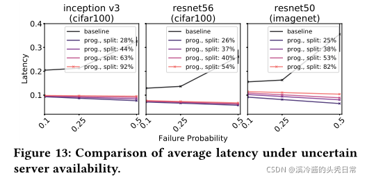
Latency comparison: In this scenario, we compareSPINNagainst a single-exit offloaded variant of the same networks. This time instead of simply failing the inference when the remote end is unavailable, we allow for retransmission with exponential backoff, a common behaviour of distributed systems to avoid channel contention. When a sample fails under the respective probability distribution, the result gets retransmitted. If the same sample fails again, the client waits double the time and retransmits, until it succeeds. Here, we assume Jetson-10W offloads to our server over 4G and varying failure probability (Pfail∈ {0.1,0.25,0.5}). The initial retransmission latency is 20 ms. We ran each experiment three times and report the mean and standard deviation of the latencies.
延迟比较:在这个场景中,我们将spinn与同一网络的单一出口卸载变体进行比较。这一次,我们不是简单地在远端不可用时失败推断,而是允许使用指数后退重传,这是分布式系统避免通道争用的常见行为。当一个样本在各自的概率分布下失败时,结果被重传。如果相同的示例再次失败,客户端将等待两倍的时间并重新传输,直到它成功。在这里,我们假设Jetson-10W在4G上卸载到我们的服务器,并且故障概率不同(Pfail∈{0.1,0.25,0.5})。初始重传延迟为20毫秒。我们对每个实验进行了三次,并报告了延迟的平均值和标准差。
As depicted in Figure 13, the non-progressive baseline follows a trajectory of increasing latency as the failure probability gets higher, due to the additional back-off latency each time a sample fails. While the impact on the average latency for both networks going from Pfail= 0.1 to Pfail= 0.25 is gradual, at 3.9%, 5.8% and 4.7% for Inception-v3, ResNet-56 and ResNet-50 respectively, the jump from Pfail= 0.25 to Pfail= 0.5 is much more dramatic, at 52.9%, 91% and 118%. The variance at Pfail= 0.5 is also noticeably higher, compared to previous values, attributed to higher number of retransmissions and thus higher discrepancies across different runs. We should note that despite the considerably higher latency of the non-progressive baseline, its accuracy can be higher, since all samples – whether re-transmitted or not – exit at the final classifier. Last, we also notice a slight reduction in the average latency of SPINN’s models as Pfailincreases. This is a result of more samples early-exiting in the network, as the server becomes unavailable more often.
如图13所示,由于每次样本失败时都会有额外的后退延迟,所以随着失败概率的增加,非渐进式基线会遵循延迟增加的轨迹。虽然从Pfail= 0.1到Pfail= 0.25对两个网络的平均延迟的影响是渐进的,对于incept -v3、ResNet-56和ResNet-50,分别为3.9%、5.8%和4.7%,但从Pfail= 0.25到Pfail= 0.5的变化则更为显著,分别为52.9%、91%和118%。与以前的值相比,Pfail= 0.5的方差也明显更高,这是由于更多的重传次数,因此不同运行之间的差异也更高。我们应该注意到,尽管非进行性基线的延迟相当高,但它的准确性可以更高,因为所有的样本——无论是否重新传输——都在最终分类器退出。最后,我们还注意到随着pfail的增加,spin模型的平均延迟略有减少。这是由于网络中出现了更多的示例,服务器变得更加不可用。
To sum up, these two results demonstrate thatSPINNcan perform sufficiently, in terms of accuracy and latency, even when the remote end remains unresponsive, by falling back to results of local exits. Compared to other systems, as the probability of failure when offloading to the server increases, there is a gradual degradation of the quality of service, instead of catastrophic unresponsiveness of the application.
综上所述,这两个结果表明,即使在远端没有响应的情况下,通过退回到本地出口的结果,spinn在准确性和延迟方面都可以充分执行。与其他系统相比,当卸载到服务器时发生故障的概率增加时,服务质量会逐渐下降,而不是应用程序灾难性的无响应。
五、讨论
SPINN and the current ML landscape. The status-quo deploy- ment process of CNNs encompasses the maintenance of two models: a large, highly accurate model on the cloud and a compact, lower-accuracy one on the device. However, this approach comes with significant deployment overheads. First, from a development time perspective, the two-model approach results in two time- and resource-expensive stages. In the first stage, the large model is designed and trained requiring multiple GPU-hours. In the second stage, the large model is compressed through various techniques in order to obtain its lightweight counterpart, with the selection and tuning of the compression method being a difficult task in itself. Furthermore, typically, to gain back the accuracy loss due to compression, the lightweight model has to be fine-tuned through a number of additional training steps.
SPINN和当前ML景观。cnn目前的部署过程包括两种模型的维护:一种是在云上的大型高精度模型,另一种是在设备上的小型高精度模型。然而,这种方法带来了巨大的部署开销。首先,从开发时间的角度来看,两模型方法导致两个时间和资源昂贵的阶段。在第一阶段,大模型的设计和训练需要多个gpu小时。在第二阶段,通过各种技术对大模型进行压缩,以获得轻量化模型,压缩方法的选择和调整本身就是一项艰巨的任务。此外,通常情况下,为了恢复由于压缩而造成的精度损失,轻量级模型必须通过一些额外的训练步骤进行微调。
With regards to the lightweight compressed networks, SPINN is orthogonal to these techniques and hence a compressed model can be combined with SPINN to obtain further gains. Given a compressed model, our system would proceed to derive a progressive inference variant with early exits and deploy the network with a tailored implementation. For use-cases where pre-trained models are employed, SPINN can also smoothly be adopted by modifying its training scheme (Section 3.2) so that the pre-trained backbone is frozen during training and only the early exits are updated.
对于轻量级压缩网络,自旋n与这些技术是正交的,因此压缩模型可以与自旋n相结合以获得进一步的收益。给定一个压缩模型,我们的系统将继续推导一个具有早期出口的渐进推理变量,并使用定制的实现部署网络。对于使用预训练模型的用例,也可以通过修改其训练方案(章节3.2)顺利采用SPINN,使预训练骨干在训练期间冻结,只更新早期出口。
Nonetheless, with SPINN we also enable an alternative paradigm that alleviates the main limitations of the current practice. SPINN requires a single network design step and a single training process which trains both the backbone network and its early exits. Upon deployment, the model’s execution is adaptively tuned based on the multiple target objectives, the environmental conditions and the device and cloud load. In this manner, SPINN enables a highly customised deployment which is dynamically and efficiently adjusted to sustain its performance in mobile settings. This approach is further supported by the ML community’s growing number of works on progressive networks [23, 35, 48, 72, 81, 83, 84] which can be directly targeted by SPINN to yield an optimised deployment on mobile platforms.
尽管如此,有了SPINN,我们还启用了另一种范式,它减轻了当前实践的主要限制。SPINN需要一个单一的网络设计步骤和一个单一的训练过程——训练主干网络和它的早期出口。在部署后,模型的执行将根据多个目标目标、环境条件、设备和云负载进行自适应调优。通过这种方式,SPINN可以实现高度定制的部署,动态有效地调整以维持其在移动设置中的性能。这种方法进一步得到了ML社区在渐进网络上越来越多的作品的支持[23,35,48,72,81,83,84],SPINN可以直接针对这些作品在移动平台上进行优化部署。
Limitations and future work.Despite the challenges addressed by SPINN, our prototype system has certain limitations. First, the scheduler does not explicitly optimise for energy or memory consumption of the client. The energy consumption could be integrated as another objective in the MOO solver of the scheduler, while memory footprint could be minimised by only loading part of the model in memory and always offloading the rest. Moreover, whileSPINN supports splitting at any given layer, we limit the candidate split points of each network to the outputs of ReLU layers, due to their high compressibility (Section 3.3). Although offloading could happen at sub-layer, filter-level granularity, this would impose extra overhead on the scheduler due to the significantly larger search space.
局限性和未来的工作。尽管SPINN解决了的挑战,我们的原型系统仍有一定的局限性。首先,调度器没有针对客户机的能量或内存消耗进行显式优化。在调度程序的MOO求解器中,可以将作为另一个目标来集成能量消耗,而内存占用可以通过只在内存中加载模型的一部分并始终卸载其余部分来最小化。此外,尽管自旋n支持在任意给定层上分裂,但由于ReLU层的高压缩性,我们将每个网络的候选分裂点限制在ReLU层的输出上(章节3.3)。尽管卸载可能发生在子层、过滤器级粒度上,但由于搜索空间很大,这将给调度器带来额外的开销。
Our workflow also assumes the model to be available at both the client and server side. While cloud resources are often dedicated to specific applications, edge resources tend to present locality challenges. To handle these, we could extend SPINN to provide incremental offloading [29] and cache popular functionality [76] closer to its users. In the future, we intend to explore multi-client settings and simultaneous asynchronous inferences on a single memory copy of the model, as well as targeting regression tasks and recurrent neural networks.
我们的工作流还假设模型在客户端和服务器端都可用。云资源通常专门用于特定的应用程序,而边缘资源往往会带来局部挑战。为了处理这些问题,我们可以扩展SPINN,以提供增量卸载[29]和更接近其用户的流行功能[76]。在未来,我们打算探索多客户端设置和同步异步推理在一个单一的记忆副本的模型,以及目标回归任务和递归神经网络。
六、结论
In this paper, we present SPINN, a distributed progressive inference engine that addresses the challenge of partitioning CNN inference across device-server setups. Through a run-time scheduler that jointly tunes the early-exit policy and the partitioning scheme, the proposed system supports complex performance goals in highly dynamic environments while simultaneously guaranteeing the robust operation of the end system. By employing an efficient multi-objective optimisation approach and a CNN-specific communication optimiser, SPINN is able to deliver higher performance over the state-of-the-art systems across diverse settings, without sacrificing the overall system’s accuracy and availability.
在这篇文章里,我们提出了SPINN,一个分布式渐进引擎,用于解决跨设备-服务器设置划分CNN推理的挑战。通过联合调优早期退出策略和划分方案的运行时调度器,所提出的系统在高度动态的环境中支持复杂的性能目标,同时保证终端系统的稳定运行。通过采用高效的多目标优化方法和专门的CNN的通信优化器,SPINN能够在不同设置的最先进的系统上提供更高的性能,而不牺牲整个系统的准确性和可用性。
