代码实现

import tensorflow as tf
import random
from tensorflow.examples.tutorials.mnist import input_data

tf.set_random_seed(777)
import matplotlib.pyplot as plt

mnist = input_data.read_data_sets("MNIST_data/", one_hot=True)

learning_rate = 0.001
train_times = 15
batch_size = 100

# 处理好保存的路径
TB_SUMMARY_DIR = './mnist'

# 占位符
X = tf.placeholder(tf.float32, [None, 784])
Y = tf.placeholder(tf.float32, [None, 10])

x_image = tf.reshape(X, [-1, 28, 28, 1])
tf.summary.image('input', x_image, 3)

keep_prob = tf.placeholder(tf.float32)

with tf.variable_scope('layer1') as scope:
    W1 = tf.get_variable('W', shape=[784, 512],
                         initializer=tf.contrib.layers.xavier_initializer())
    b1 = tf.Variable(tf.random_normal([512]))
    L1 = tf.nn.relu(tf.matmul(X, W1) + b1)
    L1 = tf.nn.dropout(L1, keep_prob)

    # 显示直方图信息
    tf.summary.histogram('X', X)
    tf.summary.histogram('weights', W1)
    tf.summary.histogram('bias', b1)
    tf.summary.histogram('layer', L1)

with tf.variable_scope('layer2') as scope:
    W2 = tf.get_variable('W', shape=[512, 512],
                         initializer=tf.contrib.layers.xavier_initializer())
    b2 = tf.Variable(tf.random_normal([512]))
    L2 = tf.nn.relu(tf.matmul(L1, W2) + b2)
    L2 = tf.nn.dropout(L2, keep_prob)

    # 显示直方图信息
    tf.summary.histogram('weights', W2)
    tf.summary.histogram('bias', b2)
    tf.summary.histogram('layer', L2)

with tf.variable_scope('layer3') as scope:
    W3 = tf.get_variable('W', shape=[512, 512],
                         initializer=tf.contrib.layers.xavier_initializer())
    b3 = tf.Variable(tf.random_normal([512]))
    L3 = tf.nn.relu(tf.matmul(L2, W3) + b3)
    L3 = tf.nn.dropout(L3, keep_prob)

    # 显示直方图信息
    tf.summary.histogram('weights', W3)
    tf.summary.histogram('bias', b3)
    tf.summary.histogram('layer', L3)

with tf.variable_scope('layer4') as scope:
    W4 = tf.get_variable('W', shape=[512, 512],
                         initializer=tf.contrib.layers.xavier_initializer())
    b4 = tf.Variable(tf.random_normal([512]))
    L4 = tf.nn.relu(tf.matmul(L3, W4) + b4)
    L4 = tf.nn.dropout(L4, keep_prob)

    # 显示直方图信息
    tf.summary.histogram('weights', W4)
    tf.summary.histogram('bias', b4)
    tf.summary.histogram('layer', L4)

with tf.variable_scope('layer5') as scope:
    W5 = tf.get_variable('W', shape=[512, 10],
                         initializer=tf.contrib.layers.xavier_initializer())
    b5 = tf.Variable(tf.random_normal([10]))
    L5 = tf.matmul(L4, W5) + b5

    # 显示直方图信息
    tf.summary.histogram('weights', W5)
    tf.summary.histogram('bias', b5)
    tf.summary.histogram('l5', L5)

cost = tf.reduce_mean(tf.nn.softmax_cross_entropy_with_logits(
    logits=L5, labels=Y
))
op = tf.train.AdamOptimizer(learning_rate).minimize(cost)

tf.summary.scalar('loss', cost)

summary = tf.summary.merge_all()

sess = tf.Session()
sess.run(tf.global_variables_initializer())

writer = tf.summary.FileWriter(TB_SUMMARY_DIR)
writer.add_graph(sess.graph)
global_step = 0

for epoch in range(train_times):
    avg_cost = 0
    n_batch = int(mnist.train.num_examples / batch_size)

    for i in range(n_batch):
        train_X, train_Y = mnist.train.next_batch(batch_size)
        feed_dict = {X: train_X, Y: train_Y, keep_prob: 0.7}
        s, _ = sess.run([summary, op], feed_dict=feed_dict)
        writer.add_summary(s, global_step=global_step)
        global_step += 1

        avg_cost += sess.run(cost, feed_dict=feed_dict)/n_batch

    print('次数', epoch + 1, '代价', avg_cost)

correct_prediction = tf.equal(tf.argmax(L5, 1), tf.argmax(Y, 1))
accurary = tf.reduce_mean(tf.cast(correct_prediction, tf.float32))
print('Accurary:', sess.run(accurary, feed_dict={X: mnist.test.images, Y: mnist.test.labels, keep_prob: 1}))

r = random.randint(0, mnist.test.num_examples - 1)
print('Labels', sess.run(tf.argmax(mnist.test.labels[r:r + 1], 1)))
print('Prediction:', sess.run(tf.argmax(L5, 1), feed_dict={X: mnist.test.images[r:r + 1], keep_prob: 1}))

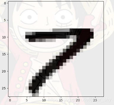
plt.imshow(mnist.test.images[r:r + 1].reshape(28, 28),
           cmap='Greys',
           interpolation='nearest')
plt.show()

结果

次数 1 代价 0.4386966144225813
次数 2 代价 0.1591908445920456
次数 3 代价 0.11683887722478678
次数 4 代价 0.09964911644855014
次数 5 代价 0.08224488782611766
次数 6 代价 0.07104504382322462
次数 7 代价 0.06707874412479051
次数 8 代价 0.05773867003535006
次数 9 代价 0.05370125422296538
次数 10 代价 0.04962954983072867
次数 11 代价 0.04811620763524181
次数 12 代价 0.04361318696713583
次数 13 代价 0.04301256288065233
次数 14 代价 0.0406030363424427
次数 15 代价 0.038484621727627406
Accurary: 0.9819
Labels [7]
Prediction: [7]