DBSCAN

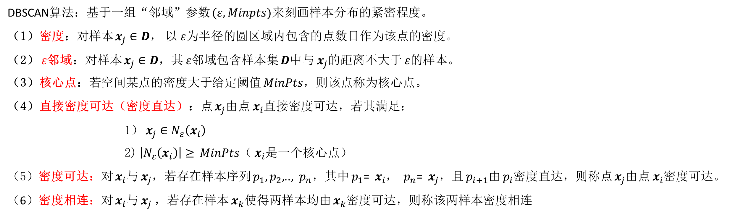
DBSCAN基本介绍

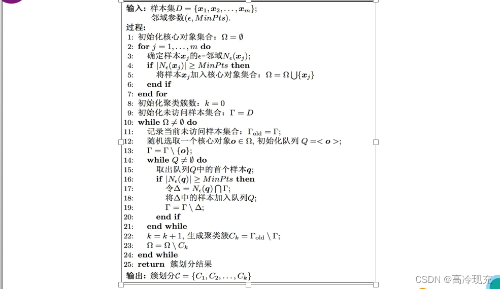
DBSCAN伪代码

DBSCAN评价

优点：
无需输入类别数𝑘，可适用于任意形状的聚类簇；
对噪声、异常点不敏感，能够识别出噪声点，不依赖于初始类中心的选取。

缺点：样本集密度不均、聚类间距差较大时，聚类结果较差；样本集较大时，收敛时间较长； 对于参数𝜀和𝑀𝑖𝑛𝑃𝑡𝑠,调参难度较大，不同参数组合对聚类结果影响较大；对于高维数据，点之间极为稀疏，密度很难定义

DBSCAN Matlab实现

function [ result ] = DBSCAN( sample, neighbor_range, MinPts )
% 每一行为一个向量
result = [];
% 存放核心对象集
core = [];
amount = size(sample, 1);
% 记录每两个节点是否邻近
record = zeros(amount);
for i = 1:amount
    temp = 0;
    for j = 1:amount
        if( j~=i && pdist(sample([i,j],:)) <= neighbor_range)
            temp = temp + 1;
            record(i, j) = 1;
        end
    end
    if( temp >= MinPts)
        core = [core i];
    end
end
core
% 聚类簇数
cluster = 0;
% notaccess记录该节点是否被访问过
notaccess = ones(amount, 1);
while(~isempty(core))
    index = randi(size(core, 1));
    % 初始化队列
    queue = core(index);
    % 从核心对象集中删除该对象
    core(index) = [];   
    notaccess(queue) = 0;
    temp_cluster = [];
%     queue
    fprintf('\n');
    while(~isempty(queue))
        temp = queue(1);
        temp_cluster = [temp_cluster temp];
        queue(1) = [];
        if(sum(record(temp, :)) >= MinPts)
            for i = 1:amount
                if(record(temp, i) && notaccess(i))
                    queue = [queue i];
                    notaccess(i) = 0; 
                    if(find(core, i))
                        core(core == i) = [];
                    end
                end
            end
        end
%         queue
%         fprintf('\n');
%         temp_cluster
%         fprintf('\n');
    end    
    cluster = cluster + 1;
    result = [result; temp_cluster];
end
% cluster
% result

end

测试用例

A=[0 2;1 1;1 2;1 3;2 2;5 5;5 4;5 6;4 5;6 5];
DBSCAN(A,1,4)

DBSCAN Python实现

import numpy as np
import queue
import random as rd


def DBSCAN(sample, neighbor_range, Minpts):
    amount = sample.shape[0]
    record = np.mat(np.zeros([amount, amount], dtype=int))
    core = []
    for i in range(0, amount):
        temp = 0
        for j in range(0, amount):
            if j == i or np.sqrt(np.sum(np.square(sample[i] - sample[j]))) > neighbor_range:
                # print('fail')
                # print(str(i) + "  " + str(j))
                # print(np.sqrt(np.sum(np.square(sample[i] - sample[j]))))
                continue
            temp = temp + 1
            # print('success')
            # print(np.sqrt(np.sum(np.square(sample[i] - sample[j]))))
            record[i, j] = 1
        if temp >= Minpts:
            core.append(i)
    print(core)
    print(record)
    cluster = 0
    notaccess = [1] * amount
    while core:
        index = rd.randint(0, len(core) - 1)
        dateque = queue.Queue()
        dateque .put(core[index])
        del core[index]
        notaccess[index] = 0
        temp_cluster = []
        while not dateque .empty():
            temp = dateque .get()
            temp_cluster.append(temp)
            if np.sum(record[temp]) >= Minpts:
                for i in range(0, amount):
                    if record[temp, i] and notaccess[temp] == 1:
                        dateque.put(i)
                        notaccess[i] = 0
                        if i in core:
                            core.remove(i)
        cluster = cluster + 1
        print("The cluster" + str(cluster) + ":")
        print(temp_cluster)


A = [[0, 2], [1, 1], [1, 2], [1, 3], [2, 2], [5, 5], [5, 4], [5, 6], [4, 5], [6, 5]]
B = np.mat(A)
DBSCAN(B, 1, 3)

层次聚类法

方法介绍

系统聚类法又常被称为谱系聚类法或分层聚类法。在聚类之前，先将每一个样本或变量都各自看成一类，计算样本之间距离，并以样本之间距离定义类之间的距离。先选择距离最近的一对合并成一个新类，计算新类与其他类之间的距离，再将距离最近的两类合并，如此持续做下去，这样就每次减少一类，直至所有的样本或变量都归为一大类为止，最后可以根据聚类的结果画出一张聚类的树形图，可以直观的反映整个聚类过程。

层次聚类法思路

基于最长距离法：
（1）置 t=0，规定样本之间的距离，此时各样本自成一类，即 $c_p$ 类与 $c_q$ 类的距离为 $D_{pq}=d_{pq}$，计算类之间距离的对称阵，记为 $R^{(t)}$
（2）选择矩阵 $R^{(t)}$ 中的最小值元素，假设为 $d_{pq}$ ，将对应的类 $c_p$ 类与 $c_q$ 合并成一类，记为 c m = { x ∣ x ∈ c p , o r , x ∈ c q } c_m=\{x|x\in c_p,or,x\in c_q\} cm​={x∣x∈cp​,or,x∈cq​} 。
（3）计算新类 $c_m$ 与其他类之间的距离
$$D_{mk}=\underset{i\in c_m,j\in c_k}{\min }{d}_{ij}=min(D_{pk},D_{qk})$$
将 $R^{(t)}$中 p,q 行, p,q列分别合并为一个新行新列，新行新列对应为类 $c_m$ ，所得到的矩阵记为 $R^{(t+1)}$ 。
（4）若全部样本已聚集成一个类，则停止算法；否则 t=t+1 ，转（2）。

算法优缺点

优点：适用于任意形状和任意属性的数据集，不需要预先设定聚类数，可以发现类的层次关系。
缺点：计算复杂度太高， 𝑂(𝑛^3)，一步错步步错。

一种实现方式

为了减少所需要的空间，这里并不使用一个距离矩阵来记录两两距离，而且即使使用矩阵，矩阵在更新时所需要做的变换也不简单。所以我干脆用字典 distance: dict来保存两两距离，字典的键为数值对 $(i,j)$，并且有 $i<j$。 另外用remain_cluster 记录可用的点，删除合并的簇，添加新的簇，都需要用到这个集合。
更新的过程以一个例子来讲，假如有1，2，3，4，5这五个点，然后我们发现1和4最近这时候我们分四步进行：

1. 在 remain_cluster 中去除1和4
2. 利用 remain_cluster计算新的距离（2，6），（3，6），（5，6）不用计算（1，6）和（4，6）因为在第一步我们就将他们删去了
3. 将 distance 中键值含有1或4的键值对删去
4. 在 remain_cluster 中添加簇6（6为簇1和簇4合并）

代码实现

# Hierarchical clustering method
import numpy as np


def Hc_method(data: list):
    data = np.array(data)
    amount = len(data)
    distance = {}
    remain_cluster = set(range(amount))
    cluster_value = [0] * (amount - 1)

    for i in range(amount - 1):
        for j in range(i + 1, amount):
            # Euclidean Distance
            distance[(i, j)] = np.sqrt(np.sum(np.square(data[i] - data[j])))
    for i in range(amount - 1):
        cluster_value[i] = min(distance.values())
        index = [k for k, v in distance.items() if v == cluster_value[i]][0]

        print("Merge " + str(i + 1) + ":")
        print(index)
        print("Distance:" + str(cluster_value[i]))

        del distance[index]
        remain_cluster.remove(index[0])
        remain_cluster.remove(index[1])
        # COMplete method(最长距离法)
        for items in remain_cluster:
            if items <= index[0] and items <= index[1]:
                distance[(items, amount + i)] = max(distance[(items, index[0])], distance[(items, index[1])])
                del distance[(items, index[0])]
                del distance[(items, index[1])]
            elif index[0] < items <= index[1]:
                distance[(items, amount + i)] = max(distance[(index[0], items)], distance[(items, index[1])])
                del distance[(index[0], items)]
                del distance[(items, index[1])]
            else:
                distance[(items, amount + i)] = max(distance[(index[0], items)], distance[(index[1], items)])
                del distance[(index[0], items)]
                del distance[(index[1], items)]
        remain_cluster.add(amount + i)
        record = set()
        for items in distance:
            if items[0] == index[0] or items[0] == index[1] or items[1] == index[0] or items[1] == index[1]:
                record.add(items)
        for elements in record:
            del distance[elements]

        print("cluster {0}: {1} + {2}".format(str(amount), str(index[0]), str(index[1])))


test_data = [[1, 2], [2, 3], [3, 4], [4, 3], [2, 5], [6, 1], [5, 5], [4, 7]]
Hc_method(test_data)

K-means法

基本原理

从直观上：离得越近的数据越相似，理应被划分为同一簇 ——数据间的相似性与它们之间的欧式距离成反比
K-means聚类是简单无监督学习算法，用于已知类数𝒌。
给定数据集 { x l } l = 1 n \{x_l\}^n_{l=1} {xl​}l=1n​，要将其划分为𝑘个簇，𝑘个簇中心记为 $c_i$ (“簇均值向量”),𝑖=1,2,…,𝑘。希望数据到它所属类中心的距离越小越好，定义如下的损失函数：
J = min ⁡ { c i , i = 1 , 2 , ⋯   , k } ∑ i = 1 k ∑ x ∈ c i ∥ x − c i ∥ 2 2 J=\min_{\{c_i,i=1,2,\cdots,k\}}\sum_{i=1}^k\sum_{x\in c_i}\|x-c_i\|^2_2 J={ci​,i=1,2,⋯,k}min​i=1∑k​x∈ci​∑​∥x−ci​∥22​
𝐽值在一定程度上刻画了簇内样本围绕簇均值向量的紧密程度， 𝐽 值越小，则簇内样本相似度越高。

K−means算法步骤（给定聚类数𝑘 ）

𝑠𝑡𝑒𝑝1：初始化，给定类数 𝑘，置 𝑗=0，从样本向量中选取任意𝑘个向量${\mathbf{c}}_1^j,{\mathbf{c}}_2^j\dots {\mathbf{c}}_k^j$作为聚类中心，并记中心为 ${\mathbf{c}}_i^j$ 的聚类块为$C_i^j$。

𝑠𝑡𝑒𝑝2：将向量样本按最短欧式距离归入𝑘聚类块。例 $x_l$ 到 $c_i^j$：
$$\Vert {\mathbf{x}}_l-{\mathbf{c}}_i^j{\Vert }_2=\underset{1\le t\le k}{\min }\Vert {\mathbf{x}}_l-{\mathbf{c}}_t^j{\Vert }_2$$
𝑠𝑡𝑒𝑝3：调整聚类中心。
$$c_i^{j+1}=\frac{{\sum }_{x_t\in c_i^j}{x}_t}{N_i}$$
，$N_i$ 为聚类块 $C_i^j$ 的向量数。

𝑠𝑡𝑒𝑝4：若𝑠𝑡𝑒𝑝2聚类中心不再明显变换则终止，否则𝑗=𝑗+1，转𝑠𝑡𝑒𝑝2。

终止迭代目标函数： J = min ⁡ { c i , i = 1 , 2 , ⋯   , k } ∑ i = 1 k ∑ x ∈ c i ∥ x − c i ∥ 2 2 J=\min_{\{c_i,i=1,2,\cdots,k\}}\sum_{i=1}^k\sum_{x\in c_i}\|x-c_i\|^2_2 J=min{ci​,i=1,2,⋯,k}​∑i=1k​∑x∈ci​​∥x−ci​∥22​

python实现

import numpy as np


def my_kmeans(data: list, k: int):
    amount = len(data)
    data = np.array(data)
    index = [0] * amount
    iter = 0
    if k > amount:
        print("Error")
        return
    cluster_center = data[0:k]
    shutdown = False
    target = 1000000

    while not shutdown and iter < 10000:
        iter += 1
        print(iter)
        internal_amount = [0] * k
        new_target = 0
        for i in range(amount):
            temp = [0] * k
            for j in range(k):
                temp[j] = np.sum(np.square(data[i] - cluster_center[j]))
            index[i] = temp.index(min(temp))
            internal_amount[index[i]] += 1
        new_cluster = np.zeros([k, len(data[0])])
        for i in range(amount):
            new_cluster[index[i]] += data[i]
        for i in range(k):
            cluster_center[i] = new_cluster[i] / internal_amount[i]
        print(cluster_center)
        for i in range(amount):
            new_target += np.sum(np.square(data[i] - cluster_center[index[i]]))
        print(new_target)
        print(index)
        if abs(target - new_target)/target < 0.001:
            shutdown = True
        else:
            target = new_target


A = [[0, 2], [5, 5], [1, 2], [1, 3], [2, 2], [1, 1], [5, 4], [5, 6], [4, 5], [6, 5]]
my_kmeans(A, 2)