网页怎么预先加载模型
深度学习 (Deep Learning)
什么是转学? (What is Transfer Learning?)
Transfer learning is a research problem in machine learning that focuses on storing knowledge gained while solving one problem and applying it to a different but related problem.
转移学习是机器学习中的一个研究问题,其重点是存储在解决一个问题并将其应用于其他但相关的问题时获得的知识。
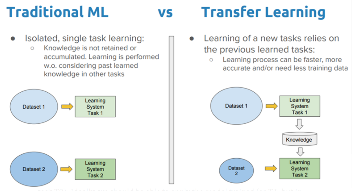
The traditional machine learning approach generalizes unseen data based on patterns learned from the training data, whereas for transfer learning, it begins from previously learned patterns to solve a different task.
传统的机器学习方法基于从训练数据中学习的模式来概括看不见的数据,而对于转移学习,它是从先前学习的模式开始以解决不同的任务 。
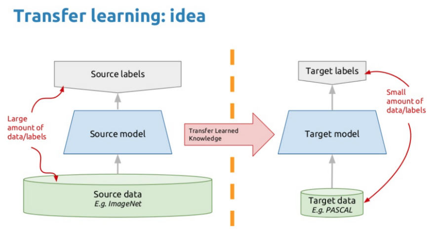
有两种常见的转移学习方法: (There are two common approaches to transfer learning:)
Developed model approach: Develop a model that is better than a naive model to ensure that some feature learning has been performed. Reuse and tune the developed model for the task of interest.
开发的模型方法:开发比单纯模型更好的模型,以确保已执行某些功能学习。 重用和调整开发模型以完成感兴趣的任务。
Pre-trained model approach: Select a pre-trained source model from available models to reuse and fine-tune.
预先训练的模型方法:从可用模型中选择一个预先训练的源模型,以进行重用和微调。
In this post, we shall focus on the pre-trained model approach as it is commonly used in the field of deep learning.
在本文中,我们将专注于深度学习领域中常用的预训练模型方法。
什么是预训练模型? (What are Pre-trained Models?)
A pre-trained model is a saved network that was previously trained on a large dataset, typically on a large-scale image-classification task. One can use the pre-trained model as it is or use transfer learning to customize this model to a given task.
预先训练的模型是一个保存的网络,以前是在大型数据集上进行训练的 ,通常是在大型图像分类任务上进行训练的 。 可以按原样使用预先训练的模型,也可以使用转移学习针对特定任务自定义此模型。
The intuition behind transfer learning is that if a model is trained on a large and general enough dataset, this model will effectively serve as a generic model of the visual world. We can then take advantage of these learned feature maps without having to start from scratch by training a large model on a large dataset.
迁移学习的直觉是, 如果在足够大且足够通用的数据集上训练模型,则该模型将有效地充当视觉世界的通用模型 。 然后,我们可以利用这些学习到的特征图,而不必通过在大型数据集上训练大型模型而从头开始。
Let’s take a deep dive into VGG16 - a notable pre-trained model submitted to the Large Scale Visual Recognition Challenge in 2014.
让我们深入研究VGG16-在2014年提交给大规模视觉识别挑战赛的 著名预训练模型。
VGG16架构 (VGG16 Architecture)
The VGG network architecture was introduced by Simonyan and Zisserman in their 2014 paper, Very Deep Convolutional Networks for Large Scale Image Recognition. This model had achieved a 92.7% top-5 test accuracy in ImageNet, which is a dataset of over 14 million images belonging to 1,000 classes. The number ‘16’ in VGG16 refers to its 16 layers which have weights. The network is considerably large with approximately 138 million parameters.
VGG网络架构由Simonyan和Zisserman在他们的2014年论文《 用于大规模图像识别的超深度卷积网络》中介绍 。 该模型在ImageNet中获得了92.7%的top-5测试准确性,该数据集包含超过1400万张图像(属于1,000个类别)。 VGG16中的数字“ 16”表示具有权重的16层。 该网络非常庞大,具有大约1.38亿个参数。
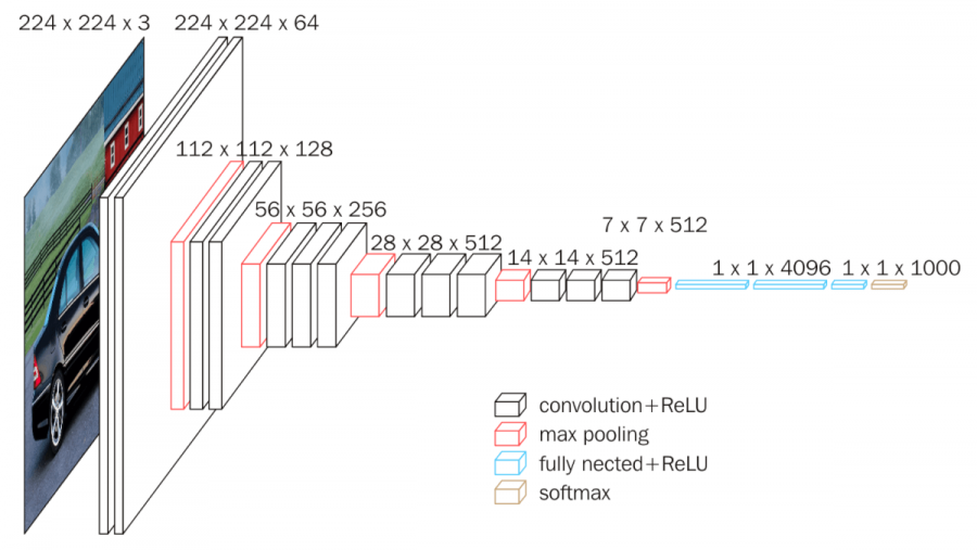

The input to conv1 layer is of fixed size 224 x 224 RGB image. The image is passed through a stack of convolutional layers, where the filters were used with a very small receptive field: 3×3 (which is the smallest size to capture the notion of left/ right, up/ down, center). In one of the configurations, it also utilizes 1×1 convolution filters, which can be seen as a linear transformation of the input channels (followed by non-linearity).
conv1层的输入具有固定大小的224 x 224 RGB图像。 图像通过一叠卷积层,在其中使用了很小的接收场的滤镜:3×3(这是捕获左/右,上/下,中心的概念的最小大小)。 在其中一种配置中,它还利用了1×1卷积滤波器,这可以看作是输入通道的线性变换(其次是非线性)。
The convolution stride is fixed to 1 pixel; the spatial padding of convolution layer input is such that the spatial resolution is preserved after convolution, i.e. the padding is 1-pixel for 3×3 convolution layers. Spatial pooling is carried out by five max-pooling layers, which follow some of the convolution layers (not all the convolution layers are followed by max-pooling). Max-pooling is performed over a 2×2 pixel window, with stride 2.
卷积步幅固定为1个像素; 卷积层输入的空间填充是这样的:在卷积后保留空间分辨率,即,对于3×3卷积层,填充为1像素。 空间池化由五个最大卷积层执行,这五个最大卷积层跟随一些卷积层(并非所有卷积层都跟随最大卷积)。 最大合并在跨度为2的2×2像素窗口上执行。
Three fully connected layers follow a stack of convolutional layers (which has a different depth in different architectures): the first two have 4,096 channels each, the third performs 1,000-way ILSVRC classification and thus contains 1,000 channels (one for each class). The final layer is the soft-max layer. The configuration of the fully connected layers is the same in all networks.
三个完全连接的层遵循一堆卷积层(在不同体系结构中深度不同):前两个分别具有4,096个通道,第三层执行1,000路ILSVRC分类,因此包含1,000个通道(每个类别一个)。 最后一层是soft-max层 。 在所有网络中,完全连接的层的配置都是相同的。
All hidden layers are equipped with the rectification (ReLU) non-linearity. It is also noted that none of the networks (except for one) contain Local Response Normalisation (LRN), such normalization does not improve the performance on the dataset, but leads to increased memory consumption and computation time.
所有隐藏层都具有整流(ReLU)非线性特性。 还应注意,除了一个网络外,没有一个网络包含本地响应规范化(LRN),这种规范化不会提高数据集的性能,但会导致内存消耗和计算时间增加。
We shall approach a problem statement and explore the basics of how transfer learning using a pre-trained model works, how to fine-tune the hyper-parameters to improve model performance, and interpret the learning curves.
我们将处理问题陈述,并探索使用预训练的模型进行转移学习的工作原理,如何微调超参数以改善模型性能以及解释学习曲线的基础知识。
问题陈述:使用迁移学习,构建卷积神经网络(“ CNN”)模型将神奇宝贝分类为各自的类别。 (Problem Statement: Using Transfer Learning, build a Convolutional Neural Network (“CNN”) model to classify Pokémons into their respective categories.)
让我们编码并抓住一切! (Let’s code and catch ‘em all!)
import os
import cv2
import requests
import numpy as np
import pandas as pd
from tensorflow import keras
from tensorflow.keras.models import Model
from tensorflow.keras import layers
from tensorflow.keras.preprocessing.image import img_to_array
from tensorflow.keras.preprocessing import image
from tensorflow.keras.utils import to_categorical
from tensorflow.keras.applications import vgg16
from tensorflow.keras.layers import Flatten, Dense, BatchNormalization, Dropout
from tensorflow.keras.optimizers import Adam
from tensorflow.keras.callbacks import ModelCheckpoint
from sklearn.model_selection import train_test_split
import scikitplot as skplt
import matplotlib.pyplot as plt
import seaborn as sns
%matplotlib inline
资料准备 (Data Preparation)
I have selected 5 categories of Pokémons from the Pokémons Dataset. Load these images and plot a bar chart to get a feel of how many images there are in each class.
我从“ 神奇宝贝”数据集中选择了5个类别的神奇宝贝 。 加载这些图像并绘制条形图,以感觉每个班级有多少图像。
path = os.getcwd() + '/pokemon dataset'


classes = os.listdir((path))
print(f'Total number of categories: {len(classes)}')


# Create a dictionary which contains class and number of images in that class
counts = {}
for i in classes:
    counts[i] = len(os.listdir(os.path.join(path, i)))

print(f'Total number of images in dataset: {sum(list(counts.values()))}')


# Plot the number of images in each class
sns.set_context('talk')
sns.set_palette(sns.color_palette('muted'))
sns.set_style('ticks')


plt.figure(figsize=(10, 5))
sns.barplot(x=list(counts.keys()), y=list(counts.values())).set_title('Number of images in each class')
plt.xticks(rotation = 90)
plt.margins(x=0)
plt.show()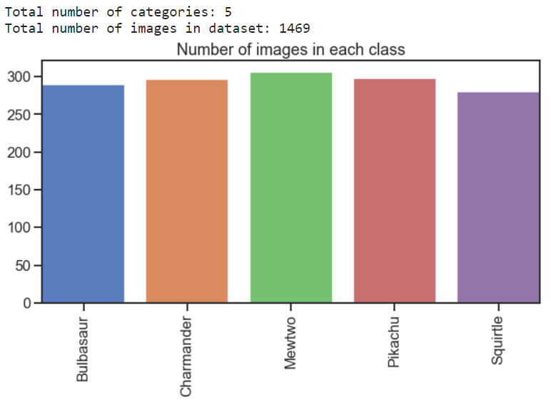
# Create dataset and sort the items in the dictionary
dataset = sorted(counts.items(), key=lambda x:x[1],reverse = True)
print(dataset)


# Extract labels
dataset = [i[0] for i in dataset]
print(dataset)
With the above bar chart, there is a good average size of at least 280 images per Pokémon class. Due to hardware constraints, we would work with an input image dimension of 128 X 128 instead of the original 224 X 224 used in the VGG16 model. We shall proceed to read, resize, and scale these images for training.
有了上面的条形图,每个神奇宝贝类别的平均大小都可以达到280张图像。 由于硬件限制,我们将使用128 X 128的输入图像尺寸,而不是VGG16模型中使用的原始224 X 224。 我们将继续阅读,调整大小和缩放这些图像以进行培训。
X = [] # Empty list for images
Y = [] # Empty list for labels


IMAGE_DIMS = (128, 128, 3) # Set image dimensions


# Loop through all classes
for c in classes:
    if c in dataset:
        dir_path = os.path.join(path, c)
        label = dataset.index(c) # the label is an index of class in data

        # Read, resize, add images and labels to lists
        for i in os.listdir(dir_path):
            image = cv2.imread(os.path.join(dir_path, i))

            try:
                resized = cv2.resize(image,(IMAGE_DIMS[0],IMAGE_DIMS[1]))
                X.append(resized)
                Y.append(label)


            except:
                print(os.path.join(dir_path, i), '[ERROR] can\'t read the file.')
                continue


# Convert list with images to numpy array and reshape it
X = np.array(X).reshape(-1, IMAGE_DIMS[0], IMAGE_DIMS[1],IMAGE_DIMS[2])


# Scale data in array
X = X / 255.0
print(X.shape)


# Convert labels to categorical format
y = to_categorical(Y, num_classes = len(dataset))
Load and split the dataset for training and testing of the CNN model. A test size of 0.2 was used, meaning 80% of the dataset would be used for training purposes while the remaining 20% serves as the testing component. We then split the dataset in a stratified fashion, using the labels, y, as the class labels. The dataset is also shuffled before splitting, to enhance the randomness of probability sampling. The random state controls the shuffling applied to the data before applying the split. An integer is passed in this parameter for reproducible output across multiple function calls.
加载和拆分数据集以进行CNN模型的训练和测试。 使用的测试大小为0.2 ,这意味着数据集的80%将用于训练目的,而其余的20%将用作测试组件。 然后,我们在一个分层的方式分割数据集,使用标签,Y,作为类的标签。 数据集在拆分之前也要进行混洗 ,以增强概率采样的随机性。 随机状态控制在应用拆分之前应用于数据的改组。 在此参数中传递整数,以便在多个函数调用之间可重现输出。
X_train, X_test, y_train, y_test = train_test_split(X, y, test_size=0.2,
                                                    stratify=y, shuffle=True, random_state=1)
使用转移学习创建CNN模型 (Creation of CNN Model using Transfer Learning)
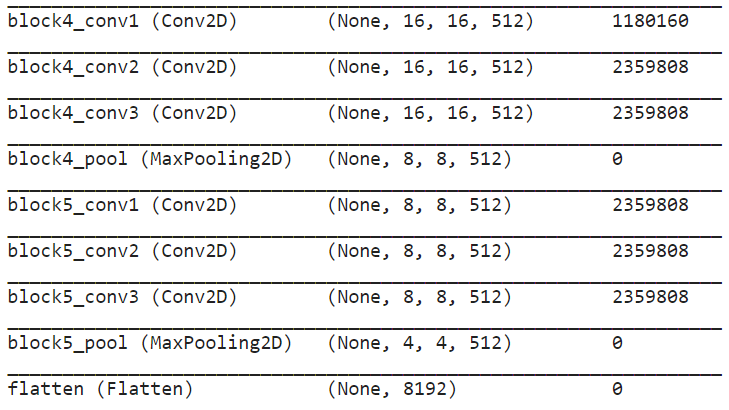
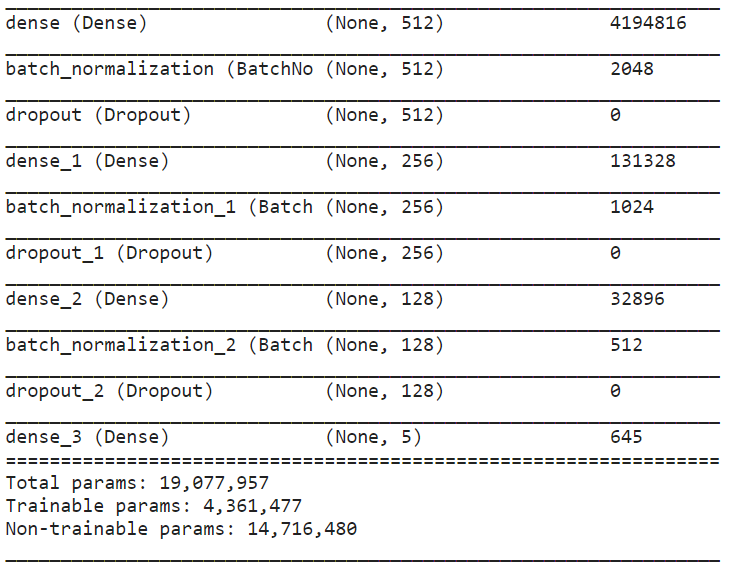
Transfer learning is applied by freezing the “deep layers” of the model and only re-training the classification layers.
通过冻结模型的“深层”并仅重新训练分类层来应用转移学习。
We have selected to use the Adam optimization, which is a stochastic gradient descent method that is based on an adaptive estimation of first-order and second-order moments.
我们选择使用Adam优化 ,它是一种基于一阶和二阶矩的自适应估计的随机梯度下降方法。
According to Kingma et al., 2014, this method is
根据Kingma等人(2014年) ,此方法是
“computationally efficient, has little memory requirement, invariant to diagonal re-scaling of gradients, and is well suited for problems that are large in terms of data/ parameters.”
“计算效率高,几乎没有存储需求,不影响梯度的对角线重新缩放,并且非常适用于数据/参数较大的问题。”
# Import VGG16 from keras with pre-trained weights that is trained on imagenet
# Include_top=False to exclude the top classification layer
# weights='imagenet' to use the weights from pre-training on Imagenet


base_model = tf.keras.applications.VGG16(include_top=False, weights='imagenet', input_shape=IMAGE_DIMS)


for layer in base_model.layers:
     layer.trainable = False

# Build the classification layers on top of the base VGG16 base layers for the dataset
model = tf.keras.Sequential(base_model.layers)


model.add(Flatten())
model.add(Dense(512, activation = 'relu'))
model.add(BatchNormalization())
model.add(Dropout(0.5))
model.add(Dense(256, activation = 'relu'))
model.add(BatchNormalization())
model.add(Dropout(0.5))
model.add(Dense(128, activation = 'relu'))
model.add(BatchNormalization())
model.add(Dropout(0.25))
model.add(Dense(len(dataset), activation = 'softmax'))


model.compile(optimizer=tf.keras.optimizers.Adam(),
              loss=keras.losses.categorical_crossentropy,
              metrics=['accuracy'])


model.summary()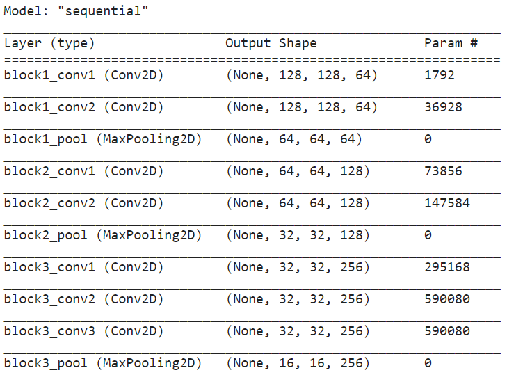
模型训练 (Model Training)
initial_epochs = 8
initial_batch_size = 32


# Enable run function eagerly to use function decorator
tf.config.experimental_run_functions_eagerly(True)


checkpoint_filepath = 'Pokemon_model.h5'


model_checkpoint_callback = tf.keras.callbacks.ModelCheckpoint(filepath=checkpoint_filepath, save_weights_only=True,
                                                               monitor='val_accuracy', mode='max', save_best_only=True)


# Save only the best model weights at the end of every epoch
history = model.fit(X_train, y_train, validation_split=0.2, epochs=initial_epochs,
                    batch_size=initial_batch_size, verbose=1,
                    callbacks=[model_checkpoint_callback])


test_loss, test_acc = model.evaluate(X_test, y_test, verbose=1)
print('test_loss:', test_loss)
print('test_acc:', test_acc)
学习曲线 (Learning Curves)
A learning curve is a plot of model learning performance over experience or time. Learning curves are a widely used diagnostic tool in machine learning for algorithms that learn from a training dataset incrementally. The model can be evaluated on the training dataset and validation dataset after each update during training, and plots of the measured performance are created to reflect the learning curves.
学习曲线是模型学习绩效随经验或时间变化的图 。 学习曲线是机器学习中广泛使用的诊断工具,用于从训练数据集中逐步学习的算法。 在训练期间的每次更新之后,可以在训练数据集和验证数据集上评估模型,并创建测量的性能图以反映学习曲线。
Reviewing learning curves of models during training can be used to diagnose problems with learning, such as an underfit or overfit model, as well as whether the training and validation datasets are suitably representative.
在训练期间查看模型的学习曲线可用于诊断学习问题,例如欠拟合或过拟合模型,以及训练和验证数据集是否具有代表性。
Train Learning Curve: Learning curve calculated from the training dataset that gives an idea of how well the model is learning.
训练学习曲线 :根据训练数据集计算出的学习曲线,可以了解模型的学习程度。
Validation Learning Curve: Learning curve calculated from a validation dataset that gives an idea of how well the model is generalizing.
验证学习曲线 :从验证数据集计算得出的学习曲线,可以了解模型的概括程度。
Let’s plot the learning curves for the training and validation accuracy/ loss.
让我们为训练和验证准确性/损失绘制学习曲线。
sns.set_context('talk')
sns.set_palette('dark')
sns.set_style('ticks')


acc = history.history['accuracy']
val_acc = history.history['val_accuracy']


loss = history.history['loss']
val_loss = history.history['val_loss']


plt.figure(figsize=(20,16))
plt.subplot(2, 1, 1)
plt.plot(acc, label='Training Accuracy')
plt.plot(val_acc, label='Validation Accuracy')
plt.legend(loc='best', shadow=True)
plt.ylabel('Accuracy')
plt.ylim([min(plt.ylim()),1])
plt.title('Training and Validation Accuracy')


plt.subplot(2, 1, 2)
plt.plot(loss, label='Training Loss')
plt.plot(val_loss, label='Validation Loss')
plt.legend(loc='best', shadow=True)
plt.ylabel('Loss')
plt.title('Training and Validation Loss')
plt.xlabel('epoch')
plt.show()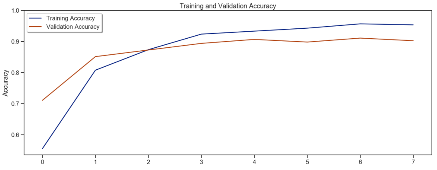
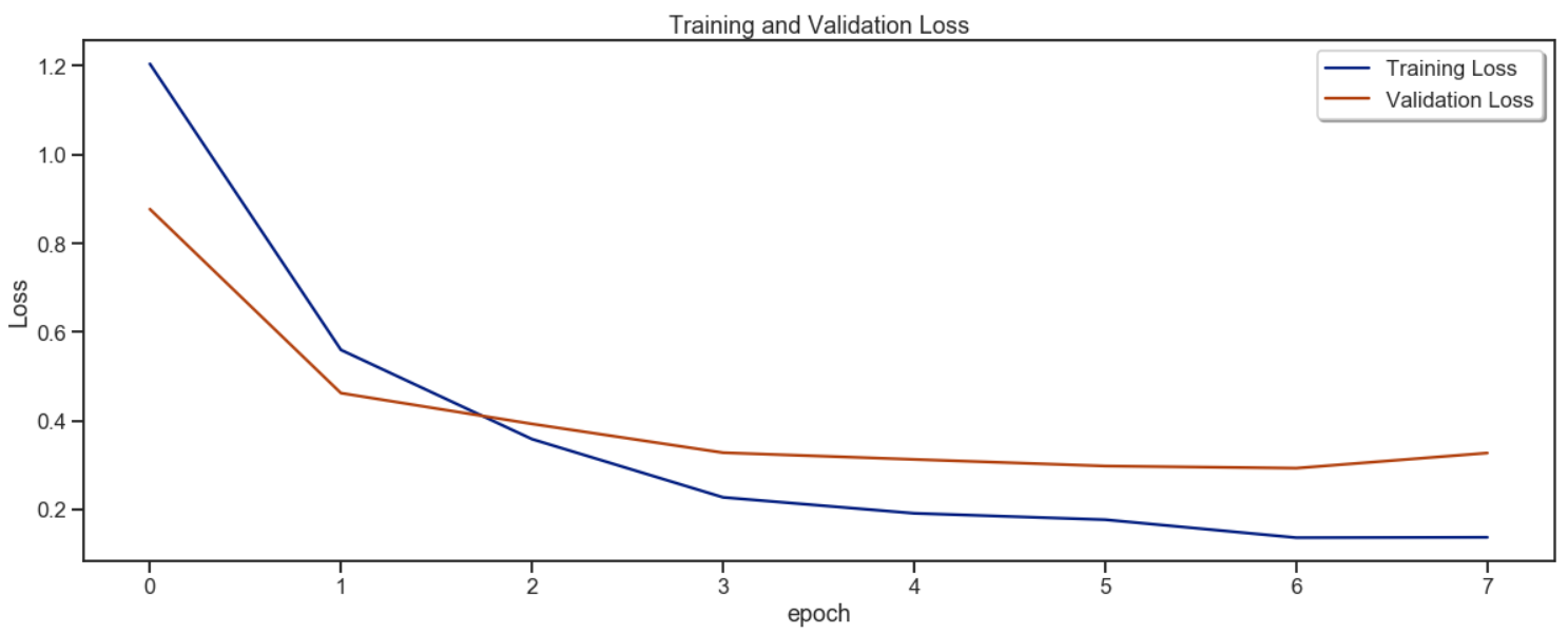
From the learning curves, as plotted, a good fit of the learning algorithm was observed. A good fit is identified by a training and validation accuracy/loss that decreases to a point of stability with a minimal gap between the two final accuracy/loss values.
如图所示,从学习曲线可以观察到学习算法的良好拟合。 训练和验证的准确性/损失会降低到稳定点,并且两个最终准确性/损失值之间的差距很小,从而可以确定良好的配合 。
The accuracy of the model will always be higher on the training dataset than the validation dataset, and vice versa, the loss of the model will almost always be lower on the training dataset than the validation dataset. This means that we should expect a generalization gap between the train and validation loss learning curves.
该模型的准确性将永远是比验证数据集中的训练数据集越高 ,反之亦然,该模型的损失几乎总是比对验证数据集训练数据集下 。 这意味着我们应该期望训练和验证损失学习曲线之间存在概括差距 。
A plot of learning curves shows a good fit if:
在以下情况下,学习曲线图显示出很好的拟合度:
- The plot of training accuracy/loss would increase/decrease to a point of stability. 训练准确性/损失图将增加/减少至稳定点。
- The plot of validation accuracy/loss would increase/decrease to a point of stability and has a small gap with the training accuracy/loss. 验证准确性/损失图将增加/减少至稳定点,并且与训练准确性/损失图之间的差距很小。
However, any continued training of a good fit will likely lead to an overfit.
但是,任何持续的良好健身训练都可能导致过度健身。
超参数的微调 (Fine-Tuning of Hyperparameter)
Next, we shall fine-tune the hyperparameter by using a much lower learning rate to improve the model performance.
接下来,我们将通过使用低得多的学习率来微调超参数以改善模型性能。
base_model = tf.keras.applications.VGG16(include_top=False, weights=None)


# The model weights (that are considered the best) are loaded into the model
model.load_weights(checkpoint_filepath)


model.compile(optimizer=tf.keras.optimizers.Adam(learning_rate=0.0001),
              loss=keras.losses.categorical_crossentropy,
              metrics=['accuracy'])


model.summary()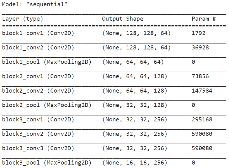
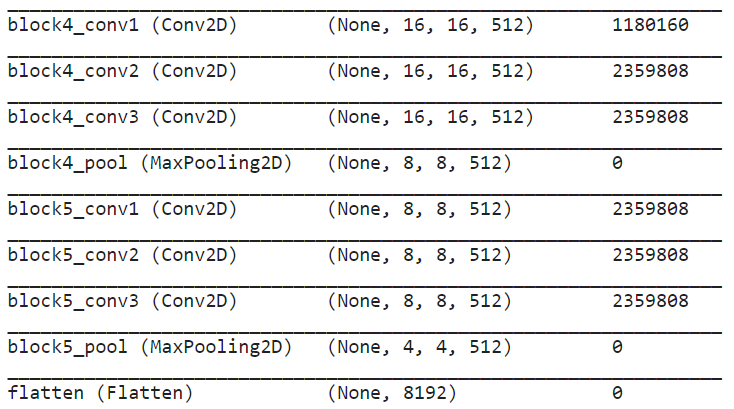
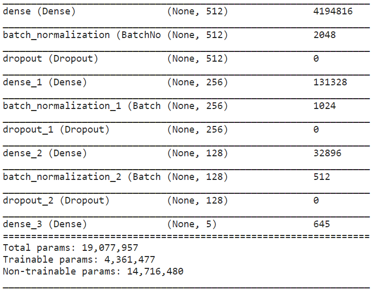
Continue training the model by increasing the number of training epochs with a decreased batch size, to improve the test accuracy and test loss.
通过增加批量减小的训练时期数继续训练模型,以提高测试准确性和测试损失。
fine_tune_epochs = 7
total_epochs =  initial_epochs + fine_tune_epochs


final_batch_size = 8


history_fine = model.fit(X_train, y_train, validation_split=0.2, epochs=total_epochs,
                         initial_epoch= history.epoch[-1], batch_size=final_batch_size, verbose=1)


test_loss_ft, test_acc_ft = model.evaluate(X_test, y_test, verbose=1)
print('test_loss_fine_tuned:', test_loss_ft)
print('test_acc_fine_tuned:', test_acc_ft)
微调后学习曲线 (Learning Curves after Fine-Tuning)
Plot learning curves of the training and validation accuracy and loss after fine-tuning to have a better visualization of how well the model was learning.
在微调后绘制训练和验证准确性以及损失的学习曲线,以更好地可视化模型的学习程度。
acc += history_fine.history['accuracy']
val_acc += history_fine.history['val_accuracy']


loss += history_fine.history['loss']
val_loss += history_fine.history['val_loss']


plt.figure(figsize=(20, 16))
plt.subplot(2, 1, 1)
plt.plot(acc, label='Training Accuracy')
plt.plot(val_acc, label='Validation Accuracy')
plt.ylabel('Accuracy')
plt.ylim([min(plt.ylim()),1])
plt.plot([initial_epochs, initial_epochs], plt.ylim(), label='Start Fine Tuning')
plt.legend(loc='best', shadow=True)
plt.title('Training and Validation Accuracy')


plt.subplot(2, 1, 2)
plt.plot(loss, label='Training Loss')
plt.plot(val_loss, label='Validation Loss')
plt.ylim([0, 1.5])
plt.ylabel('Loss')
plt.plot([initial_epochs,initial_epochs], plt.ylim(), label='Start Fine Tuning')
plt.legend(loc='best', shadow=True)
plt.title('Training and Validation Loss')
plt.xlabel('epoch')
plt.show()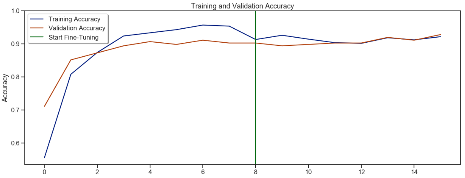
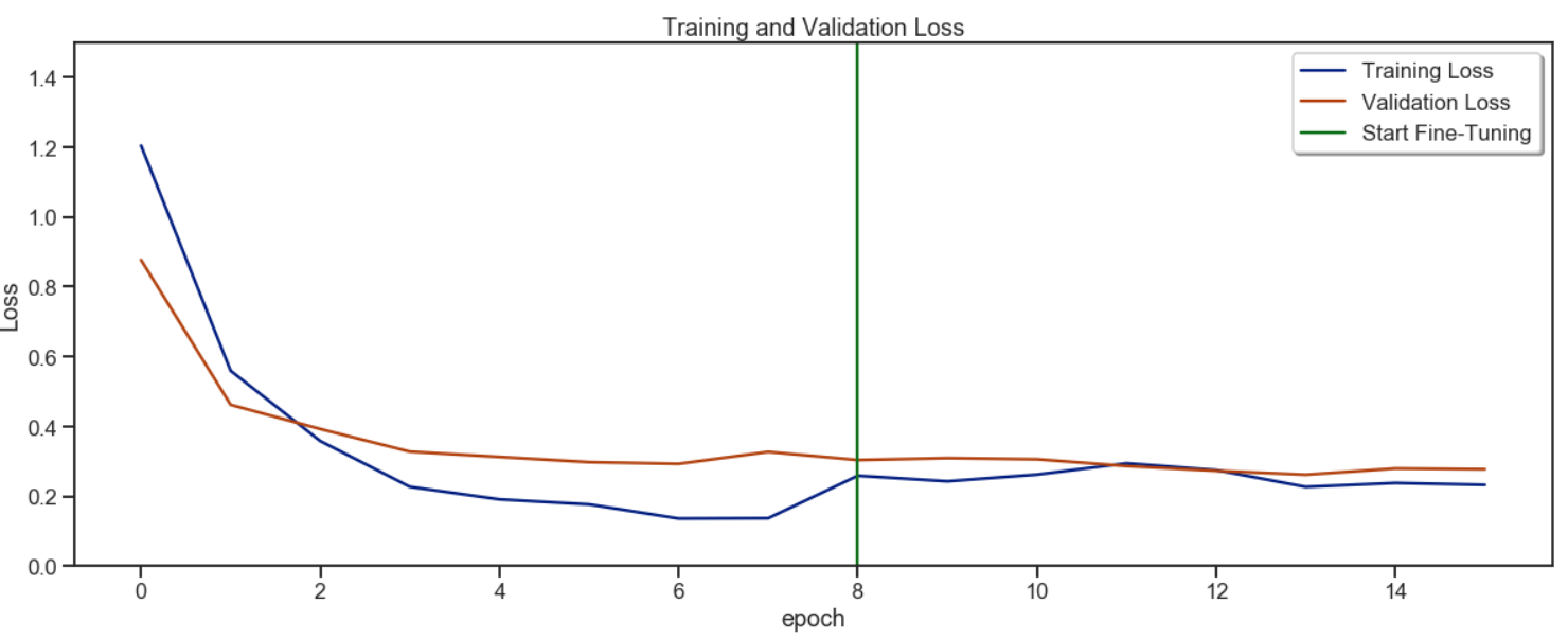
By using a slower learning rate, it has helped to improve the validation accuracy and lower the validation losses. Note that the generalization gap between the train and validation accuracy/loss learning curves have been significantly minimized.
通过使用较低的学习速度,它有助于提高验证准确性并降低验证损失。 请注意,训练与验证准确性/损失学习曲线之间的泛化差距已大大缩小。
结果评估 (Evaluation of Results)
To provide an independent evaluation of the trained model, a test dataset of unseen data was created by selecting random images of each class from the internet.
为了提供对经过训练的模型的独立评估,通过从互联网上选择每个类别的随机图像来创建看不见数据的测试数据集。
mewtwo = ['https://cdn.bulbagarden.net/upload/thumb/7/78/150Mewtwo.png/250px-150Mewtwo.png',
         'https://cdn.vox-cdn.com/thumbor/sZPPvUyKyF97UEU-nNtVnC3LpF8=/0x0:1750x941/1200x800/filters:focal(878x316:1158x596)/cdn.vox-cdn.com/uploads/chorus_image/image/63823444/original.0.jpg',
         'https://images-na.ssl-images-amazon.com/images/I/61j5ozFjJ0L._SL1024_.jpg']


pikachu = ['https://lh3.googleusercontent.com/proxy/DrjDlKlu9YonKbj3iNCJNJ3DGqzy9GjeXXSUv-TcVV4UN9PMCAM5yIkGLPG7wYo3UeA4sq5OmUWM8M6K5hy2KOAhf8SOL3zPH3axb2Xo3HX2XTU8M2xW4X6lVg=w720-h405-rw',
          'https://giantbomb1.cbsistatic.com/uploads/scale_medium/0/6087/2437349-pikachu.png',
          'https://johnlewis.scene7.com/is/image/JohnLewis/237525467']


charmander = ['https://img.pokemondb.net/artwork/large/charmander.jpg',
             'https://www.pokemoncenter.com/wcsstore/PokemonCatalogAssetStore/images/catalog/products/P5073/701-03990/P5073_701-03990_01.jpg',
             'https://cdn.vox-cdn.com/thumbor/JblVKwBfJ9BDIQJ30sfZp93QGYE=/0x0:2040x1360/1200x800/filters:focal(857x517:1183x843)/cdn.vox-cdn.com/uploads/chorus_image/image/61577305/jbareham_180925_ply0802_0024.0.jpg']


bulbasaur = ['https://img.pokemondb.net/artwork/large/bulbasaur.jpg',
            'https://ae01.alicdn.com/kf/HTB1aWullxSYBuNjSsphq6zGvVXaR/Big-Size-55-CM-Plush-Toy-Squirtle-Bulbasaur-Charmander-Toy-Sleeping-Pillow-Doll-For-Kid-Birthday.jpg',
            'https://cdn.bulbagarden.net/upload/thumb/f/f7/Bulbasaur_Detective_Pikachu.jpg/250px-Bulbasaur_Detective_Pikachu.jpg']


squirtle = ['https://assets.pokemon.com/assets/cms2/img/pokedex/full/007.png',
           'https://cdn.vox-cdn.com/thumbor/l4cKX7ZWargjs-zlxOSW2WZVgfI=/0x0:2040x1360/1200x800/filters:focal(857x517:1183x843)/cdn.vox-cdn.com/uploads/chorus_image/image/61498573/jbareham_180925_ply0802_0030.1537570476.jpg',
           'https://thumbor.forbes.com/thumbor/960x0/https%3A%2F%2Fblogs-images.forbes.com%2Fdavidthier%2Ffiles%2F2018%2F07%2FSquirtle_Squad.jpg']


test_df = [mewtwo, pikachu, charmander, bulbasaur, squirtle]
# Empty lists to store our future data
val_x = []
val_y = []
for i, urls in enumerate(test_df):
for url in urls:
r = requests.get(url, stream = True).raw
image = np.asarray(bytearray(r.read()), dtype="uint8")
image = cv2.imdecode(image, cv2.IMREAD_COLOR)
val_x.append(image)
val_y.append(i)
rows = 5
cols = 3
fig = plt.figure(figsize = (25, 30))
for i, j in enumerate(zip(val_x, val_y)): # i - for subplots
orig = j[0] # Original, not resized image
label = j[1] # Label for that image
image = cv2.resize(orig, (IMAGE_DIMS[0], IMAGE_DIMS[1])) # Resize image
image = image.reshape(-1, IMAGE_DIMS[0], IMAGE_DIMS[1],IMAGE_DIMS[2])/255.0 # Reshape and scale resized image
preds = model.predict(image) # Predict image
pred_class = np.argmax(preds) # Define predicted class
true_label = f'True class: {dataset[label]}'
pred_label = f'Predicted: {dataset[pred_class]} {round(preds[0][pred_class]*100, 2)}%'
fig.add_subplot(rows, cols, i+1)
plt.imshow(orig[:, :, ::-1])
plt.title(f'{true_label}\n{pred_label}', fontsize=22)
plt.axis('off')
plt.tight_layout()
The above results have indicated a good performance of the trained model in terms of correctly identifying each pokémon to its respective classes. Well, with the exception of the poor Detective Pikachu, which was unfortunately identified as a Mewtwo with a prediction rate of 58.9%. Perhaps Mewtwo has decided to strike back since its movie - Pokémon: Mewtwo Strikes Back — Evolution.
以上结果表明,在正确识别每个神奇宝贝所属类别后,训练模型具有良好的性能。 好吧,除了可怜的侦探皮卡丘,不幸的是,皮卡丘被认为是猫鼬,预测率为58.9%。 自从电影《 神奇宝贝:喵喵回击-进化》以来,喵喵已经决定进行反击 。
结论 (Conclusion)
Overall, a CNN model has been successfully built using transfer learning to classify the categories from the Pokémon dataset.
总体而言,已经使用转移学习成功地构建了CNN模型,以对Pokémon数据集中的类别进行分类。
To further enhance the accuracy level of images with background noises, improvements can be made where the CNN model is trained with a large and general enough dataset. The use of transfer learning enables one to take advantage of the previously learned feature maps without having to start from scratch by training a large model on a large dataset.
为了进一步提高具有背景噪声的图像的准确度,可以在使用足够大和足够通用的数据集训练CNN模型的情况下进行改进。 转移学习的使用使人们可以利用先前学习的特征图,而不必通过在大型数据集上训练大型模型而从头开始。
网页怎么预先加载模型