文章目录
FCOS: Fully Convolutional One-Stage Object Detection
Zhi Tian, Chunhua Shen ICCV, 2019 PDF | code
Abstract
由于去除了预先定义的锚框,FCOS 减轻了计算负担并且减少了模型的超参数。By eliminating the predefined set of anchor boxes, FCOS completely avoids the complicated computation related to anchor boxes such as calculating overlapping during training. More importantly, we also avoid all hyper-parameters related to anchor boxes, which are often very sensitive to the final detection performance.
1. Introduction
目前主流的检测器(Faster R-CNN, SSD and YOLOv2, v3)依赖于预先定义的锚框,并且很长时间以来检测器的成果被归因于锚框的使用。但是,锚框的使用也带来了些固有的缺陷:
All current mainstream detectors such as Faster R-CNN, SSD and YOLOv2, v3 rely on a set of pre-defined anchor boxes and it has long been believed that the use of anchor boxes is the key to detectors’ success. Despite their great success, it is important to note that anchor-based detectors suffer some drawbacks:
- 检测器的性能对锚框的参数设置很敏感(大小、长宽比、数量)例:RetinaNet在coco数据集上通过调节参数增加了4%的mAP值。(detection performance is sensitive to the sizes, aspect ratios and number of anchor boxes.)
- 不管如何设计参数,锚框的比例和长宽比保持固定,检测器还是很难检测形变较大的物体,尤其是小物体。需要事先设定的锚框也阻碍了检测器的泛化能力,因为检测任务对象的大小和长宽比发生变化,就需要对锚框进行重新设计。(Even with careful design, because the scales and aspect ratios of anchor boxes are keptfixed, detectors encounter difficulties to deal with object candidates with large shape variations, particularly for small objects. The pre-defined anchor boxes also hamper the generalization ability of detectors, as they need to be re-designed on new detection tasks with different object sizes or aspect ratios.)
- 为了获得提高的召回率,检测器需要在输入图像上设置极为密集的锚框(一个
800x800图像在FPN网络上有超过180k数量的锚框),这也导致了正负样本的极度不均衡。(In order to achieve a high recall rate, an anchor-based detector is required to densely place anchor boxes on the input image (e.g., more than 180K anchor boxes in feature pyramid networks (FPN) [14] for an image with its shorter side being 800). Most of these anchor boxes are labelled as negative samples during training. The excessive number of negative samples aggravates the imbalance between positive and negative samples in training.) - 锚框也带来了额外的计算负担,例如交兵比的计算。(Anchor boxes also involve complicated computation such as calculating the intersection-over-union (IoU) scores with ground-truth bounding boxes.)
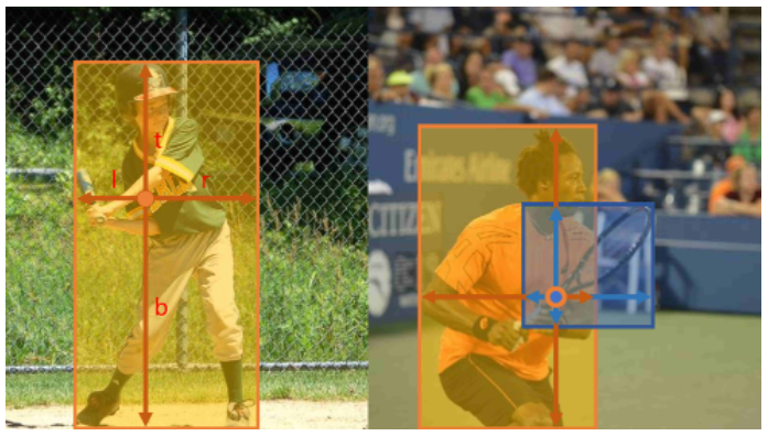
2015 CVPR年的DensenBox也尝试使用Anchor-Free的方法进行目标检测,但是DensenBox(also see this)存在两个设计上的缺陷:将输入图像剪切到一定大小(对于不需要对图像进行剪切操作的FCNs-base方法),当边界框高度重叠时导致检测不准确。In the literature, some works attempted to leverage the FCNs-based framework for object detection such as DenseBox (also see this). Specifically, these FCN-based frameworks directly predict a 4D vector plus a class category at each spatial location on a level of feature maps. However, to handle the bounding boxes with different sizes, DenseBox crops and resizes training images to afixed scale. Thus DenseBox has to perform detection on image pyramids, which is against FCN’s philosophy of computing all convolutions once. As shown in Fig. 1 (right), the highly overlapped bounding boxes result in an intractable ambiguity: it is not clear w.r.t. which bounding box to regress for the pixels in the overlapped regions.
为了解决模型会在远离目标对象中心的位置产生许多低质量的预测边界框,FCOS引入了center-ness branch降低这些低质量边界框的权重,这也是这篇论文与同年在CVPR发表的FSAF(also see this)的不同之处。In the sequel, we take a closer look at the issue and show that with FPN this ambiguity can be largely eliminated. As a result, our method can already obtain comparable detection accuracy with those traditional anchor based detectors. Furthermore, we observe that our method may produce a number of low-quality predicted bounding boxes at the locations that are far from the center of an target object. In order to suppress these low-quality detections, we introduce a novel “center-ness” branch (only one layer) to predict the deviation of a pixel to the center of its corresponding bounding box, as defined in
c
e
n
t
e
r
n
e
s
s
∗
=
min
(
l
∗
,
r
∗
)
max
(
l
∗
,
r
∗
)
×
min
(
t
∗
,
b
∗
)
max
(
t
∗
,
b
∗
)
\displaystyle centerness ^{*}=\sqrt{\frac{\min \left(l^{*}, r^{*}\right)}{\max \left(l^{*}, r^{*}\right)} \times \frac{\min \left(t^{*}, b^{*}\right)}{\max \left(t^{*}, b^{*}\right)}}
centerness∗=max(l∗,r∗)min(l∗,r∗)×max(t∗,b∗)min(t∗,b∗). This score is then used to down-weight low-quality detected bounding boxes and merge the detection results in NMS. The simple yet effective center-ness branch allows the FCN-based detector to outperform anchor-based counterparts under exactly the same training and testing settings.
作者提出的FCOS有如下优点:This new detection framework enjoys the following advantages.
-
模型与全卷积任务兼容,从而更容易重用这些任务中的想法(更容易多任务学习的方法)。Detection is now unified with many other FCN solvable tasks such as semantic segmentation, making it easier to re-use ideas from those tasks.
-
基于
Anchor-Free的模型减少了模型的超参数,使模型更简单了。Detection becomes proposal free and anchor free, which significantly reduces the number of design parameters. The design parameters typically need heuristic tuning and many tricks are involved in order to achieve good performance. Therefore, our new detection framework makes the detector, particularly its training, considerably simpler. -
基于
Anchor-Free的模型减轻了计算负担(交并比计算和边界框匹配),减少了内存占用。By eliminating the anchor boxes, our new detector completely avoids the complicated computation related to anchor boxes such as the IOU computation and matching between the anchor boxes and ground-truth boxes during training, resulting in faster training and testing as well as less training memory footprint than its anchor-based counterpart. -
取得了SOTA,并且可以应用在两阶段的模型上。Without bells and whistles, we achieve state-of-theart results among one-stage detectors. We also show that the proposed FCOS can be used as a Region Proposal Networks (RPNs) in two-stage detectors and can achieve significantly better performance than its anchor-based RPN counterparts. Given the even better performance of the much simpler anchor-free detector, we encourage the community to rethink the necessity of anchor boxes in object detection, which are currently considered as the de facto standard for detection.
-
模型可以轻易迁移到其他任务上。The proposed detector can be immediately extended to solve other vision tasks with minimal modification, including instance segmentation and key-point detection. We believe that this new method can be the new baseline for many instance-wise prediction problems.
2. Related Work
作者提及了几个Anchor-Based(Faster R-CNN, YOLO V2)和几个Anchor-Free(CornerNet, DenseBox)的方法,这里就不展开了,有兴趣的读者可以看看原论文。
3. Our Approach
In this section, we first reformulate object detection in a per-pixel prediction fashion. Next, we show that how we make use of multi-level prediction to improve the recall and resolve the ambiguity resulted from overlapped bounding boxes. Finally, we present our proposed “center-ness” branch, which helps suppress the low-quality detected bounding boxes and improves the overall performance by a large margin.
3.1. Fully Convolutional One-Stage Object Detector
| Describe | Symbol |
|---|---|
| 第 i i i个特征层 | F i ∈ R H × W × C F_{i} \in \mathbb{R}^{H \times W \times C} Fi∈RH×W×C |
| 第 i i i个特征层之前所有层的总步幅 | s s s |
| ground-truth bounding boxes | { B i } \left\{B_{i}\right\} {Bi}, where B i = ( x 0 ( i ) , y 0 ( i ) , x 1 ( i ) y 1 ( i ) , c ( i ) ) ∈ R 4 × { 1 , 2 … C } B_{i}=\left(x_{0}^{(i)}, y_{0}^{(i)}, x_{1}^{(i)} y_{1}^{(i)}, c^{(i)}\right) \in \mathbb{R}^{4} \times\{1,2 \ldots C\} Bi=(x0(i),y0(i),x1(i)y1(i),c(i))∈R4×{1,2…C} |
gt 边界框左上和右下坐标 | ( x 0 ( i ) , y 0 ( i ) ) \left(x_{0}^{(i)}, y_{0}^{(i)}\right) (x0(i),y0(i)) and ( x 1 ( i ) y 1 ( i ) ) \left(x_{1}^{(i)} y_{1}^{(i)}\right) (x1(i)y1(i)) |
gt 边界框标签 | c ( i ) c^{(i)} c(i) |
对于特征层
F
i
F_i
Fi上的每一个坐标
(
x
,
y
)
(x,y)
(x,y),都可以将其映射到输入图像的坐标
(
⌊
s
2
⌋
+
x
s
,
⌊
s
2
⌋
+
y
s
)
\left(\left\lfloor\frac{s}{2}\right\rfloor+x s,\left\lfloor\frac{s}{2}\right\rfloor+y s\right)
(⌊2s⌋+xs,⌊2s⌋+ys),靠近该位置的
(
x
,
y
)
(x,y)
(x,y)感受野的中心。Anchor-Based的检测器将输入图像上的位置视为anchor box的中心,并以这些anchor box为参考回归目标边界框,我们直接回归该位置的目标边界框。换句话说,Anchor-Free检测器直接将该位置视为训练样本,而不是基于锚的检测器中的锚框。
Specifically, location ( x , y ) (x, y) (x,y) is considered as a positive sample if it falls into any ground-truth box and the class label c ∗ c^∗ c∗ of the location is the class label of the ground-truth box. Otherwise it is a negative sample and c ∗ = 0 c^∗ = 0 c∗=0 (background class). Besides the label for classification, we also have a 4 D 4D 4D real vector t ∗ = ( l ∗ , t ∗ , r ∗ , b ∗ ) {\bf t}^∗ = (l^∗, t^∗, r^∗, b^∗) t∗=(l∗,t∗,r∗,b∗) being the regression targets for the location. Here l ∗ l^∗ l∗, t ∗ t^∗ t∗, r ∗ r^∗ r∗ and b ∗ b^∗ b∗ are the distances from the location to the four sides of the bounding box, as shown in Fig. 1 (left). If a location falls into multiple bounding boxes, it is considered as an ambiguous sample. We simply choose the bounding box with minimal area as its regression target. In the next section, we will show that with multi-level prediction, the number of ambiguous samples can be reduced significantly and thus they hardly affect the detection performance. Formally, if location ( x , y ) (x, y) (x,y) is associated to a bounding box B i B_i Bi, the training regression targets for the location can be formulated as,
l
∗
=
x
−
x
0
(
i
)
,
t
∗
=
y
−
y
0
(
i
)
r
∗
=
x
1
(
i
)
−
x
,
b
∗
=
y
1
(
i
)
−
y
\begin{aligned} l^{*} &=x-x_{0}^{(i)}, \quad t^{*}=y-y_{0}^{(i)} \\ r^{*} &=x_{1}^{(i)}-x, \quad b^{*}=y_{1}^{(i)}-y \end{aligned}
l∗r∗=x−x0(i),t∗=y−y0(i)=x1(i)−x,b∗=y1(i)−y
It is worth noting that FCOS can leverage as many foreground samples as possible to train the regressor. It is different from anchor-based detectors, which only consider the anchor boxes with a highly enough IOU with ground-truth boxes as positive samples. We argue that it may be one of the reasons that FCOS outperforms its anchor-based counterparts.
Network Outputs. Corresponding to the training targets, the final layer of our networks predicts an 80D (coco dataset 有80个种类) vector p \bf p p of classification labels and a 4D vector t = ( l , t , r , b ) {\bf t} = (l, t, r, b) t=(l,t,r,b) bounding box coordinates.
Loss Function. We define our training loss function as follows:
L
(
{
p
x
,
y
}
,
{
t
x
,
y
}
)
=
1
N
pos
∑
x
,
y
L
c
l
s
(
p
x
,
y
,
c
x
,
y
∗
)
+
λ
N
pos
∑
1
{
c
x
,
y
∗
>
0
}
L
r
e
g
(
t
x
,
y
,
t
x
,
y
∗
)
L\left(\left\{\boldsymbol{p}_{x, y}\right\},\left\{\boldsymbol{t}_{x, y}\right\}\right) =\frac{1}{N_{\text {pos }}} \sum_{x, y} L_{\mathrm{cls}}\left(\boldsymbol{p}_{x, y}, c_{x, y}^{*}\right)+\frac{\lambda}{N_{\text {pos }}} \sum \mathbb{1}_{\left\{c_{x, y}^{*}>0\right\}} L_{\mathrm{reg}}\left(\boldsymbol{t}_{x, y}, \boldsymbol{t}_{x, y}^{*}\right)
L({px,y},{tx,y})=Npos 1x,y∑Lcls(px,y,cx,y∗)+Npos λ∑1{cx,y∗>0}Lreg(tx,y,tx,y∗)
Inference. The inference of FCOS is straightforward. Given an input images, we forward it through the network and obtain the classification scores
p
x
,
y
{\bf p}_{x,y}
px,y and the regression prediction
t
x
,
y
{\bf t}_{x,y}
tx,y for each location on the feature maps
F
i
F_i
Fi. We choose the location with
p
x
,
y
>
0.05
p_{x,y} > 0.05
px,y>0.05 as positive samples.
3.2. Multi-level Prediction with FPN for FCOS
Here we show that how two possible issues of the proposed FCOS can be resolved with multi-level prediction with FPN.
- The large stride (e.g., 16×) of thefinal feature maps in a CNN can result in a relatively low best possible recall (BPR). For anchor based detectors, low recall rates due to the large stride can be compensated to some extent by lowering the required IOU scores for positive anchor boxes. For FCOS, at thefirst glance one may think that the BPR can be much lower than anchor-based detectors because it is impossible to recall an object which no location on thefinal feature maps encodes due to a large stride. Here, we empirically show that even with a large stride, FCN-based FCOS is still able to produce a good BPR, and it can even better than the BPR of the anchor-based detector RetinaNet in the official implementation Detectron (refer to Table 1). Therefore, the BPR is actually not a problem of FCOS. Moreover, with multi-level FPN prediction, the BPR can be improved further to match the best BPR the anchor-based RetinaNet can achieve.
- Overlaps in ground-truth boxes can cause intractable ambiguity , i.e., which bounding box should a location in the overlap regress? This ambiguity results in degraded performance of FCN-based detectors. In this work, we show that the ambiguity can be greatly resolved with multi-level prediction, and the FCN-based detector can obtain on par, sometimes even better, performance compared with anchor-based ones.
Following FPN, we detect different sizes of objects on different levels of feature maps. Specifically, we make use of five levels of feature maps defined as
P
3
,
P
4
,
P
5
,
P
6
,
P
7
{P_3, P_4, P_5, P_6, P_7}
P3,P4,P5,P6,P7.
P
3
P_3
P3,
P
4
P_4
P4 and
P
5
P_5
P5 are produced by the backbone CNNs’ feature maps
C
3
C_3
C3,
C
4
C_4
C4 and
C
5
C_5
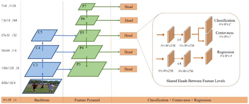
C5 followed by a 1 × 1 convolutional layer with the top-down connections in FPN, as shown in Fig. 2.
P
6
P_6
P6 and
P
7
P_7
P7 are produced by applying one convolutional layer with the stride being 2 on
P
5
P_5
P5 and
P
6
P6
P6, respectively. As a result, the feature levels
P
3
P_3
P3,
P
4
P_4
P4,
P
5
P_5
P5,
P
6
P_6
P6 and
P
7
P_7
P7 have strides 8, 16, 32, 64 and 128, respectively.
Unlike anchor-based detectors, which assign anchor boxes with different sizes to different feature levels, we directly limit the range of bounding box regression for each level. More specifically, we firstly compute the regression targets l ∗ l^∗ l∗, t ∗ t^∗ t∗, r ∗ r^∗ r∗ and b ∗ b^∗ b∗ for each location on all feature levels. Next, if a location satisfies max ( l ∗ , t ∗ , r ∗ , b ∗ ) > m i \max(l^∗, t^∗, r^∗, b^∗) > m_i max(l∗,t∗,r∗,b∗)>mi or m a x ( l ∗ , t ∗ , r ∗ , b ∗ ) < m i − 1 max(l^∗, t^∗, r^∗, b^∗) < m_{i−1} max(l∗,t∗,r∗,b∗)<mi−1, it is set as a negative sample and is thus not required to regress a bounding box anymore. Here mi is the maximum distance that feature level i needs to regress. In this work, m 2 m_2 m2, m 3 m_3 m3, m 4 m_4 m4, m 5 m_5 m5, m 6 m_6 m6 and m 7 m_7 m7 are set as 0, 64, 128, 256, 512 and ∞ \infty ∞, respectively. Since objects with different sizes are assigned to different feature levels and most overlapping happens between objects with considerably different sizes. If a location, even with multi-level prediction used, is still assigned to more than one ground-truth boxes, we simply choose the ground-truth box with minimal area as its target. As shown in our experiments, the multi-level prediction can largely alleviate the aforementioned ambiguity and improve the FCN-based detector to the same level of anchor-based ones.
Finally, following FPN, we share the heads between different feature levels, not only making the detector parameter-efficient but also improving the detection performance. However, we observe that different feature levels are required to regress different size range (e.g., the size range is [ 0 , 64 ] [0, 64] [0,64] for P 3 P_3 P3 and [ 64 , 128 ] [64, 128] [64,128] for P 4 P_4 P4), and therefore it is not reasonable to make use of identical heads for different feature levels. As a result, instead of using the standard e x p ( x ) exp(x) exp(x), we make use of e x p ( s i x ) exp(s_ix) exp(six) with a trainable scalar s i s_i si to automatically adjust the base of the exponential function for feature level P i P_i Pi, which slightly improves the detection performance.
3.3. Center-ness for FCOS
在 FCOS 中使用多级预测后,FCOS 和Anchor-Based检测器之间仍然存在性能差距。作者观察到这是由于远离对象中心的位置产生了许多低质量的预测边界框。
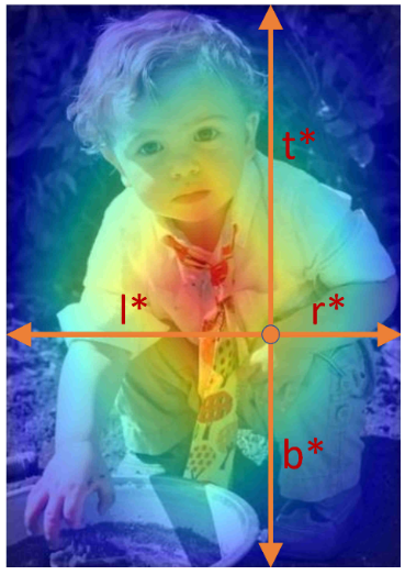
作者提出了一种简单而有效的策略来抑制这些检测到的低质量边界框,而无需引入任何超参数。具体来说,我们添加了一个单层分支,与分类分支并行(如Figure2所示)来预测位置的“中心度”。中心度描述了从该位置到该位置负责的对象中心的归一化距离,如 Figure3 所示。给定一个位置的回归目标
l
∗
l^∗
l∗,
t
∗
t^∗
t∗,
r
∗
r^∗
r∗ and
b
∗
b^∗
b∗ ,中心目标定义为,
centerness
∗
=
min
(
l
∗
,
r
∗
)
max
(
l
∗
,
r
∗
)
×
min
(
t
∗
,
b
∗
)
max
(
t
∗
,
b
∗
)
\text { centerness }^{*}=\sqrt{\frac{\min \left(l^{*}, r^{*}\right)}{\max \left(l^{*}, r^{*}\right)} \times \frac{\min \left(t^{*}, b^{*}\right)}{\max \left(t^{*}, b^{*}\right)}}
centerness ∗=max(l∗,r∗)min(l∗,r∗)×max(t∗,b∗)min(t∗,b∗)
加入中心度损失之后的总损失为:
L
(
{
p
x
,
y
}
,
{
t
x
,
y
}
)
=
1
N
pos
∑
x
,
y
L
c
l
s
(
p
⃗
x
,
y
,
c
x
,
y
∗
)
+
λ
1
N
pos
∑
x
,
y
1
c
x
,
y
∗
>
0
L
r
e
g
(
t
⃗
x
,
y
,
t
x
,
y
∗
)
+
λ
2
N
pos
∑
x
,
y
1
c
x
,
y
∗
>
0
L
c
e
n
t
e
r
−
n
e
s
s
(
centerness
x
,
y
,
centerness
x
,
y
∗
)
=
1
N
pos
∑
x
,
y
L
c
l
s
(
p
⃗
x
,
y
,
c
x
,
y
∗
)
+
λ
1
N
pos
∑
x
,
y
1
c
x
,
y
∗
>
0
L
r
e
g
(
t
⃗
x
,
y
,
t
x
,
y
∗
)
+
λ
2
N
pos
∑
x
,
y
1
c
x
,
y
∗
>
0
L
c
e
n
t
e
r
−
n
e
s
s
(
centerness
x
,
y
,
centerness
x
,
y
∗
)
\begin{aligned} \begin{aligned} L\left(\left\{\boldsymbol{p}_{x, y}\right\},\left\{\boldsymbol{t}_{x, y}\right\}\right) =& \frac{1}{N_{\text {pos }}} \sum_{x, y} L_{c l s}\left(\vec{p}_{x, y}, c_{x, y}^{*}\right)+\\ & \frac{\lambda_{1}}{N_{\text {pos }}} \sum_{x, y} \mathbb{1}_{c_{x, y}^{*}>0} L_{reg}\left(\vec{t}_{x, y}, t_{x, y}^{*}\right)+\\ & \frac{\lambda_{2}}{N_{\text {pos }}} \sum_{x, y} \mathbb{1}_{c_{x, y}^{*}>0} L_{center-ness}\left(\text { centerness }_{x, y}, \text { centerness }_{x, y}^{*}\right) \end{aligned}=& \frac{1}{N_{\text {pos }}} \sum_{x, y} L_{c l s}\left(\vec{p}_{x, y}, c_{x, y}^{*}\right)+\\ & \frac{\lambda_{1}}{N_{\text {pos }}} \sum_{x, y} \mathbb{1}_{c_{x, y}^{*}>0} L_{reg}\left(\vec{t}_{x, y}, t_{x, y}^{*}\right)+\\ & \frac{\lambda_{2}}{N_{\text {pos }}} \sum_{x, y} \mathbb{1}_{c_{x, y}^{*}>0} L_{center-ness}\left(\text { centerness }_{x, y}, \text { centerness }_{x, y}^{*}\right) \end{aligned}
L({px,y},{tx,y})=Npos 1x,y∑Lcls(px,y,cx,y∗)+Npos λ1x,y∑1cx,y∗>0Lreg(tx,y,tx,y∗)+Npos λ2x,y∑1cx,y∗>0Lcenter−ness( centerness x,y, centerness x,y∗)=Npos 1x,y∑Lcls(px,y,cx,y∗)+Npos λ1x,y∑1cx,y∗>0Lreg(tx,y,tx,y∗)+Npos λ2x,y∑1cx,y∗>0Lcenter−ness( centerness x,y, centerness x,y∗)