一般来说，我们研究分析一些海温或者降水等要素的的变化规律时，通常会进行季节特征变化分析，这就需要我们绘制不同季节的空间分布图来进行分析，这就需要我们掌握子图的绘制方法。

一般这种我们可以通过设置不同的ax进行绘制，简单介绍在这篇博客中：进阶绘图–axes

• 通过对于每个子图的不同命令，可以绘制填色图、折线图等等，这种方法的不好的地方在于需要多次重复一些语句设置，比如地形、坐标、标签等等，当然，如果不怕麻烦也可以忽略。
• 对于不同的子图，只需要对于不同的ax进行不同的绘图即可，同时对于不同的子图属性设置也要对应不同的ax序号，如果你第一个字图的ax是ax1，那么所有关于这个子图的命令语句，都要以ax1开头。
• 下面给出一个通过ax命令海温的季节空间分布图绘制的例子：

ax绘制不同子图

# -*- coding: utf-8 -*-
"""
Created on Thu Aug 12 22:20:52 2021

@author: 纪
"""
## 导入库
import cartopy.feature as cfeature
from cartopy.util import add_cyclic_point
from cartopy.mpl.ticker import LongitudeFormatter, LatitudeFormatter
import matplotlib.pyplot as plt
import numpy as np
import cartopy.crs as ccrs
import xarray as xr
## 路径
path='D:\\sst.nc'
### =================================================================
# 准备数据、选择区域、求季节平均
###==================================================================
sst=xr.open_dataset(path)
lon=sst.lon
lat=sst.lat
lat_range = lat[(lat>-22.5) & (lat<22.5)]
sst_region =sst.sel(lat=lat_range,lon=lon)
season =sst_region.groupby(
    'time.season').mean('time', skipna=True)
#=====================draw==============================================
fig=plt.figure(figsize=(20,12))#设置一个画板，将其返还给fig
###=================设置全局字体、字体大小==============================
plt.rcParams['font.family'] = 'Times New Roman'
plt.rcParams['font.size'] = 15
###=========================绘制第一个子图=================================
ax = fig.add_subplot(4, 1, 1, projection=ccrs.PlateCarree(central_longitude =180))

### 添加地形，并且设置陆地为白色遮盖
ax.add_feature(cfeature.NaturalEarthFeature('physical', 'land', '50m', \
                             edgecolor='white',facecolor='white',zorder=2))
### 添加循环，为了避免经线180°出现白色竖线                         
cycle_sst, cycle_lon = add_cyclic_point(season.sst[1], coord=lon)
cycle_LON, cycle_LAT = np.meshgrid(cycle_lon, lat_range)
### 绘制填色图   
cb=ax.contourf(cycle_LON,cycle_LAT, cycle_sst,levels=np.arange(20,36),cmap='bwr',\
   zorder=0,transform= ccrs.PlateCarree())
### 设置横纵坐标的范围  
ax.set_xticks(np.arange(0, 361, 30),crs=ccrs.PlateCarree())
ax.set_yticks(np.arange(-20, 40, 20),crs=ccrs.PlateCarree())
ax.xaxis.set_major_formatter(LongitudeFormatter(zero_direction_label =False))#经度0不加标识
ax.yaxis.set_major_formatter(LatitudeFormatter())
### 绘制等值线
contour = ax.contour(lon,lat_range, season.sst[1],colors='k',zorder=1,transform= ccrs.PlateCarree())
#zorder 显示图层叠加顺序
### 设置坐标轴的轴长、宽、离轴的距离、
ax.tick_params(which='major', direction='out', length=10, width=0.99, pad=0.2, bottom=True, left=True, right=False, top=False)
### 设置子图的标题
ax.set_title('JJA-SST horizontal distribution')
### 设置子图的colorbar
cbar = fig.colorbar(cb,shrink=0.7,ticks=[20,25,30],pad=0.04,aspect=3.5)
###=========================绘制第2个子图=================================
ax1 = fig.add_subplot(4, 1, 2, projection=ccrs.PlateCarree(central_longitude=180))#中心线为180°
ax1.add_feature(cfeature.NaturalEarthFeature('physical', 'land', '110m', \
                                            edgecolor='black', facecolor='white'))
cycle_sst1, cycle_lon = add_cyclic_point(season.sst[2], coord=lon)
cb=ax1.contourf(cycle_LON,cycle_LAT, cycle_sst1,levels=np.arange(20,34),cmap='bwr',\
    zorder=0,transform= ccrs.PlateCarree() )
contour = plt.contour(cycle_LON,cycle_LAT, cycle_sst1,colors='k',zorder=1,transform= ccrs.PlateCarree())
ax1.add_feature(cfeature.NaturalEarthFeature('physical', 'land', '50m', \
                                           edgecolor='white', facecolor='white',zorder=2))
ax1.tick_params(which='major', direction='out', length=10, width=0.99, pad=0.2, bottom=True, left=True, right=False, top=False)
ax1.set_xticks(np.arange(0, 361, 30),crs=ccrs.PlateCarree())
ax1.set_yticks(np.arange(-20, 40, 20),crs=ccrs.PlateCarree())
ax1.xaxis.set_major_formatter(LongitudeFormatter(zero_direction_label =False))#经度0不加标识
ax1.yaxis.set_major_formatter(LatitudeFormatter())
ax1.set_title('MAM-SST horizontal distribution')
cbar = fig.colorbar(cb,shrink=0.7,ticks=[20,25,30],pad=0.04,aspect=3.5)
###=========================绘制第3个子图=================================
ax2= fig.add_subplot(4, 1, 3, projection=ccrs.PlateCarree(central_longitude=180))#中心线
ax2.add_feature(cfeature.NaturalEarthFeature('physical', 'land', '110m', \
                                            edgecolor='black', facecolor='white'))
cycle_sst2, cycle_lon = add_cyclic_point(season.sst[3], coord=lon)
cb=ax2.contourf(cycle_LON,cycle_LAT, cycle_sst2,levels=np.arange(20,34),cmap='bwr',\
   zorder=0,transform= ccrs.PlateCarree()  )
contour = plt.contour(cycle_LON,cycle_LAT, cycle_sst2,colors='k',zorder=1,transform= ccrs.PlateCarree())
ax2.add_feature(cfeature.NaturalEarthFeature('physical', 'land', '50m', \
 edgecolor='white', facecolor='white',zorder=2))
ax2.tick_params(which='major', direction='out', length=10, width=0.99, pad=0.2, bottom=True, left=True, right=False, top=False)
ax2.set_xticks(np.arange(0, 361, 30),crs=ccrs.PlateCarree())
ax2.set_yticks(np.arange(-20, 40, 20),crs=ccrs.PlateCarree())
ax2.xaxis.set_major_formatter(LongitudeFormatter(zero_direction_label =False))#经度0不加标识
ax2.yaxis.set_major_formatter(LatitudeFormatter())
ax2.set_title('SON-SST horizontal distribution')
cbar = fig.colorbar(cb,shrink=0.7,ticks=[20,25,30],pad=0.04,aspect=3.5)
###=========================绘制第4个子图=================================
ax3= fig.add_subplot(4, 1, 4, projection=ccrs.PlateCarree(central_longitude=180))#中心线
ax3.add_feature(cfeature.NaturalEarthFeature('physical', 'land', '110m', \
                                            edgecolor='black', facecolor='white'))
cycle_sst3, cycle_lon = add_cyclic_point(season.sst[0], coord=lon)
cb=ax3.contourf(cycle_LON,cycle_LAT, cycle_sst3,levels=np.arange(20,34),cmap='bwr',\
    zorder=0,transform= ccrs.PlateCarree() )
contour = plt.contour(cycle_LON,cycle_LAT, cycle_sst3,colors='k',zorder=1,transform= ccrs.PlateCarree())
ax3.add_feature(cfeature.NaturalEarthFeature('physical', 'land', '50m', \
                                            edgecolor='white', facecolor='white',zorder=2))
ax3.tick_params(which='major', direction='out', length=10, width=0.99, pad=0.2, bottom=True, left=True, right=False, top=False)
ax3.set_xticks(np.arange(0, 361, 30),crs=ccrs.PlateCarree())
ax3.set_yticks(np.arange(-20, 40, 20),crs=ccrs.PlateCarree())
ax3.xaxis.set_major_formatter(LongitudeFormatter(zero_direction_label =False))#经度0不加标识
ax3.yaxis.set_major_formatter(LatitudeFormatter())
ax3.set_title('DJF-SST horizontal distribution')
cbar = fig.colorbar(cb,shrink=0.7,ticks=[20,25,30],pad=0.04,aspect=3.5)
### 保存图片到指定路径
#fig.savefig('D:\\desktopppp\\picture\\'+'SST_horizontal_distribution.tiff',format='tiff',dpi=150)

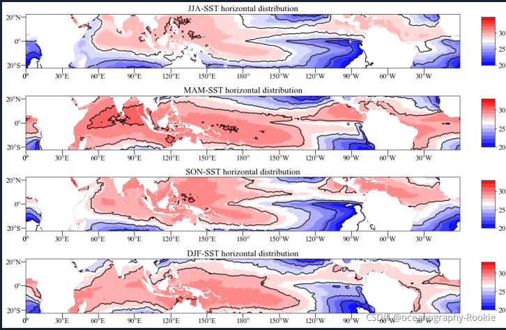
绘图结果如下，海温的四个季节的空间水平分布：

通过绘图函数封装绘制不同子图

其实，通过上面的代码，我们可以发现，有部分代码完全是重复设置的，非常的麻烦，所以我们完全可以设置一个绘图函数，减少我们的代码量。
下面给出一个使用代码封装后的绘图例子，可以前后对比一下：

"""
Created on Thu Nov  4 19:47:58 2021

@author: (ji)

E-mail : [email protected]

Introduction: keep learning
"""
import cartopy.feature as cfeature
from cartopy.mpl.ticker import LongitudeFormatter, LatitudeFormatter
import matplotlib.pyplot as plt
import numpy as np
import cartopy.crs as ccrs
import xarray as xr

path2='D:\\sst.nc'
ds=xr.open_dataset(path2).sortby("lat", ascending= True)
sst=ds.sel(lat=slice(-20,20),time=slice('2010','2010'))
season =sst.groupby('time.season').mean('time', skipna=True)
def make_map(ax, title):
    # set_extent  set crs
    ax.set_extent(box, crs=ccrs.PlateCarree())
    land = cfeature.NaturalEarthFeature('physical',
                                        'land',
                                        scale,
                                        edgecolor='white', 
                                        facecolor='white',
                                        zorder=2)
    ax.add_feature(land)  # set land color
    ax.coastlines(scale)  # set coastline resolution
    # set coordinate axis
    ax.set_xticks(np.arange(0, 360+30, 30),crs=ccrs.PlateCarree())
    ax.set_yticks(np.arange(-20, 30, 10),crs=ccrs.PlateCarree())
    ax.xaxis.set_major_formatter(LongitudeFormatter(zero_direction_label =False))#经度0不加标识
    ax.yaxis.set_major_formatter(LatitudeFormatter())
    # plt.tick_params(labelsize=25)
    lon_formatter = LongitudeFormatter(zero_direction_label=False)  
    # zero_direction_label set 0 without E or W
    lat_formatter = LatitudeFormatter()
    ax.xaxis.set_major_formatter(lon_formatter)
    ax.yaxis.set_major_formatter(lat_formatter)
    ax.set_title(title, fontsize=25, loc='center')
    ax.tick_params(which='major', 
                    direction='out', 
                    length=8,
                    width=0.99, 
                    pad=0.2, 
                    labelsize=20,
                    bottom=True, left=True, right=False, top=False)
    return ax

# # prepare 
box = [0, 361, -20, 20]  
scale = '50m'            
xstep, ystep = 30, 5   
cmap=plt.get_cmap('bwr')#'RdYlBu_r'
levels=np.arange(20,34)
zorder=0
# name=['DJF-SST horizontal distribution','JJA-SST horizontal distribution',\
#       'MAM-SST horizontal distribution','SON-SST horizontal distribution']
sea=['JJA','MAM','SON','DJF']
#=================draw   picture   =================================
fig=plt.figure(figsize=(20,12))#设置一个画板，将其返还给fig
plt.rcParams['font.family'] = 'Times New Roman'
plt.rcParams['font.size'] = 15
proj=ccrs.PlateCarree(central_longitude=180)
count=0
for i in range(len(sea)):
    count+=1

    ax=fig.add_subplot(4,1,count,projection=proj)
    make_map(ax,sea[i]+'-SST horizontal distribution')
    plot=ax.contourf(sst.lon,sst.lat,season.sel(season=sea[i]).sst,cmap=cmap,levels=levels,\
                      zorder=0,transform=ccrs.PlateCarree())
    contour=ax.contour(sst.lon,sst.lat,season.sel(season=sea[i]).sst,colors='k',zorder=1,transform=ccrs.PlateCarree())
    # pcolor=ax.pcolormesh(sst.lon,sst.lat,season.sst[i],transform=ccrs.PlateCarree(),\
    #                  cmap='bwr', zorder=0)
    # fig.colorbar(pcolor,ax=ax,shrink=0.7,ticks=[20,25,30],pad=0.04,aspect=3.5)
    fig.colorbar(plot,ax=ax,shrink=0.7,ticks=[20,25,30],pad=0.04,aspect=3.5)
plt.show()
# fig.savefig('G:\\daily\\'+'SST_horizontal_distribution.tiff',format='tiff',dpi=150)

结果是一样的：

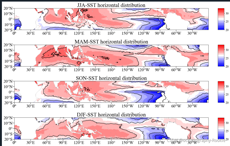
可以明显的发现，代码更简洁了，也可以将这个封装函数进行保存，以后直接导入这个函数，大大节省我们绘图时间！！！
有兴趣的小伙伴们可以尝试一下~

测试数据有点大，不方面传在这里，有需要的找我要

						    			一个努力学习python的海洋
					                    水平有限，欢迎指正！！！
				                        欢迎评论、收藏、点赞、转发、关注。
				                        关注我不后悔，记录学习进步的过程~~