7. Model Validation

Why Model Validation?
We have seen so far Various metrics(e.g., accuracy, F-measure, RMSE, …) and Evaluation protocol setups (Split Validation, Cross Validation, and Special protocols for time series)

7.1 Overfitting

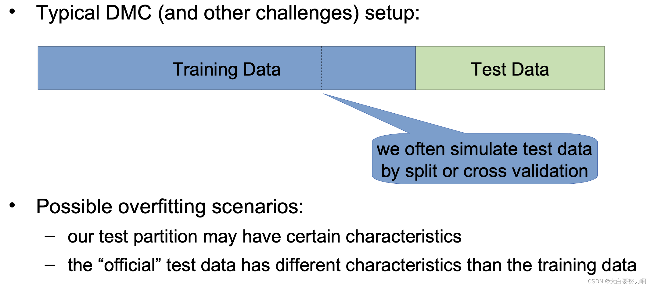
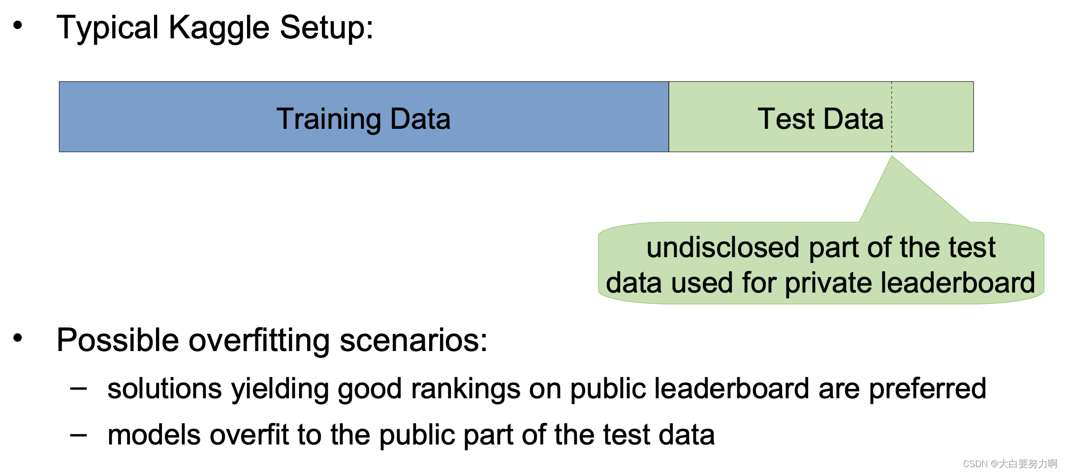
Data Mining Competitions often have a hidden test set
Ranking on public test set and ranking on hidden test set may differ

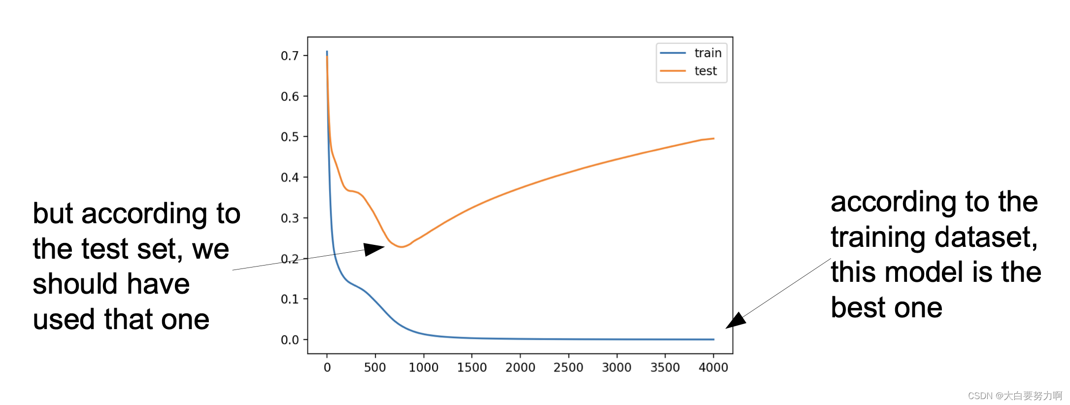
We have come across this problem quite a few times - overfitting
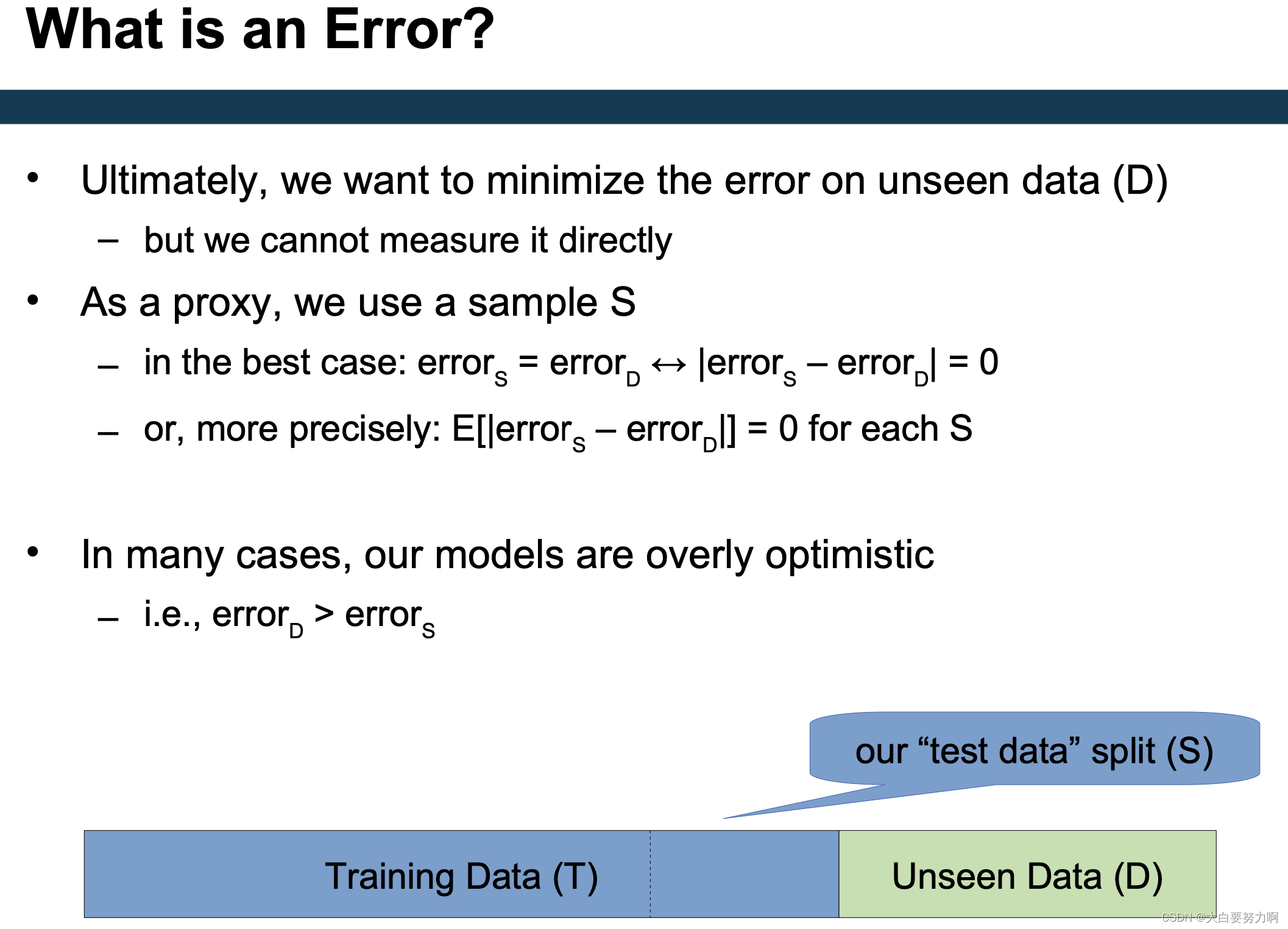
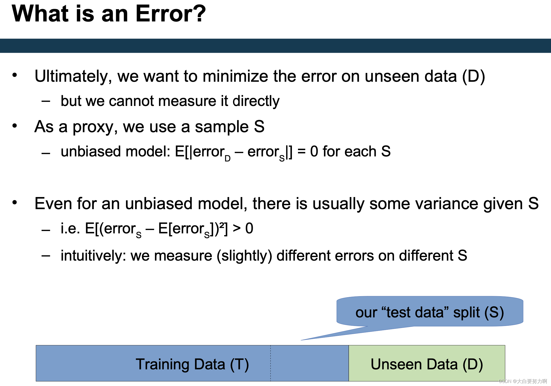
Problem: we don’t know the error on the (hidden) test set

Overfitting Revisited

Some flavors of overfitting are more subtle than others
Obvious overfitting: use test partition for training

Less obvious overfitting: tune parameters against test partition & select “best” approach based on test partition, also: by repeated submission to leaderboard

Even less obvious overfitting: use test partition in feature construction, for features such as avg. sales of product per day, avg. orders by customer, computing trends.

If we have test data without labels, we can still look at predictions – do they look somehow reasonable?

7.2 Overtuning

In academia,
-> many fields have their established benchmarks
-> achieving outstanding scores on those is required for publication
-> interesting novel ideas may score suboptimally. -> hence, they are not published
-> intensive tuning is required for publication -> hence, available compute power often beats good ideas

That “leaderboardism” has been criticized recently

In real world projects
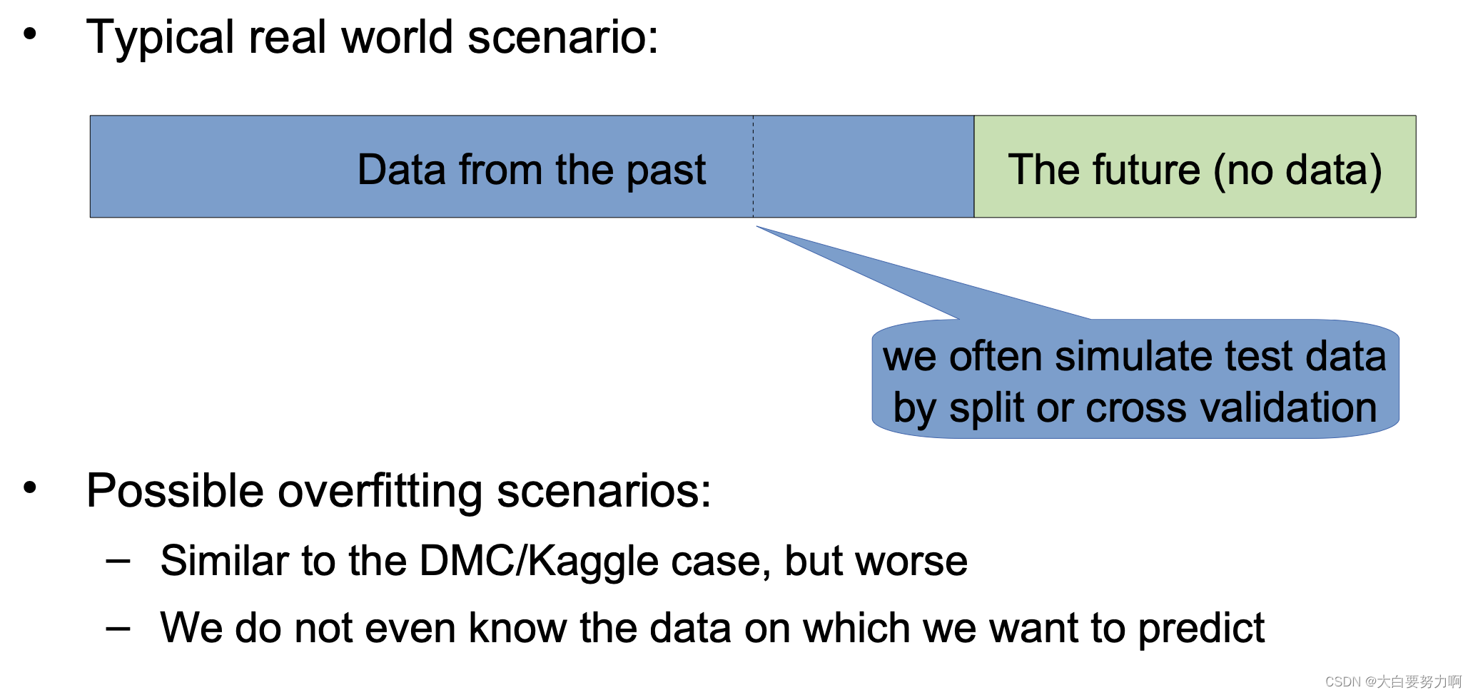
-> models overfit to past data
-> performance on unseen data is often overestimated, i.e., customers are disappointed
-> changing characteristics in data may be problematic
drift: e.g., predicting battery lifecycles
events not in training data: e.g., predicting sales for next month
-> cold start problem
some instances in the test set may be unknown before, e.g., predicting product sales for new products

7.3 Confidence Intervals for Models

Validating and Comparing Models
When is a model good? i.e., is it better than random?
When is a model really better than another one? i.e., is the performance difference by chance or by design?

Confidence Intervals for Models
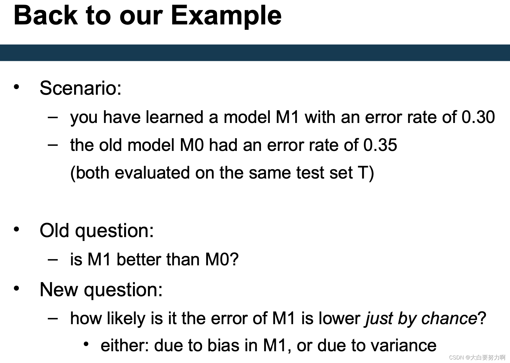
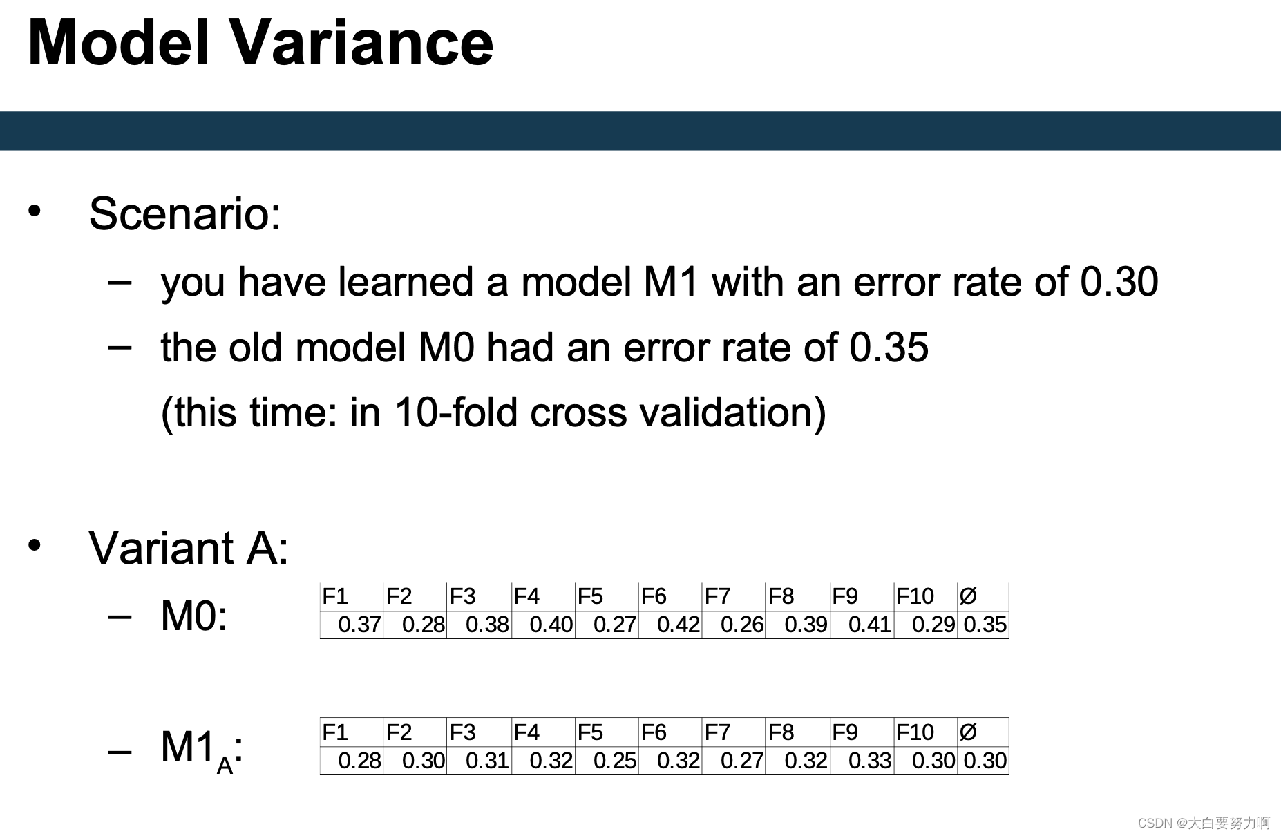
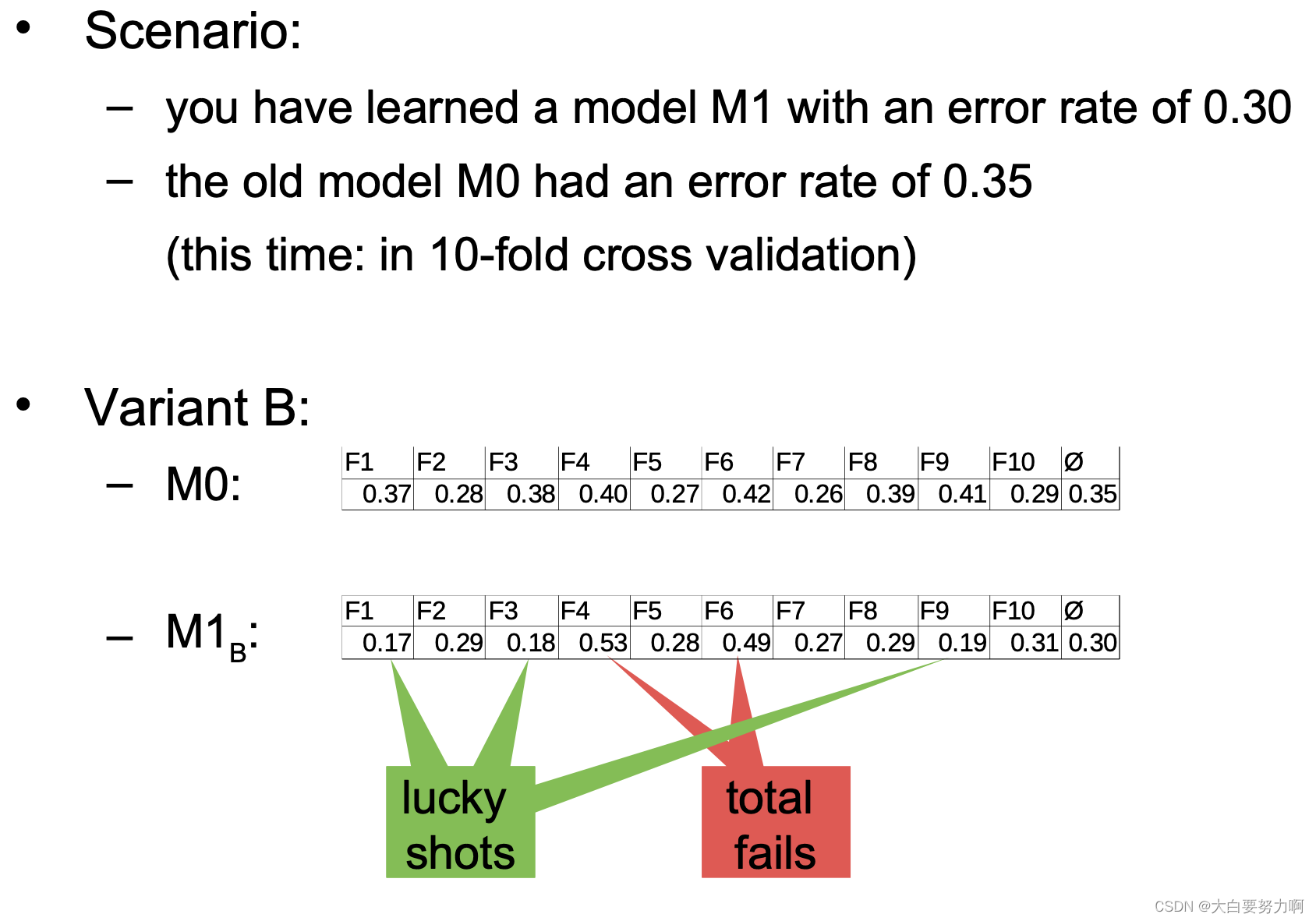
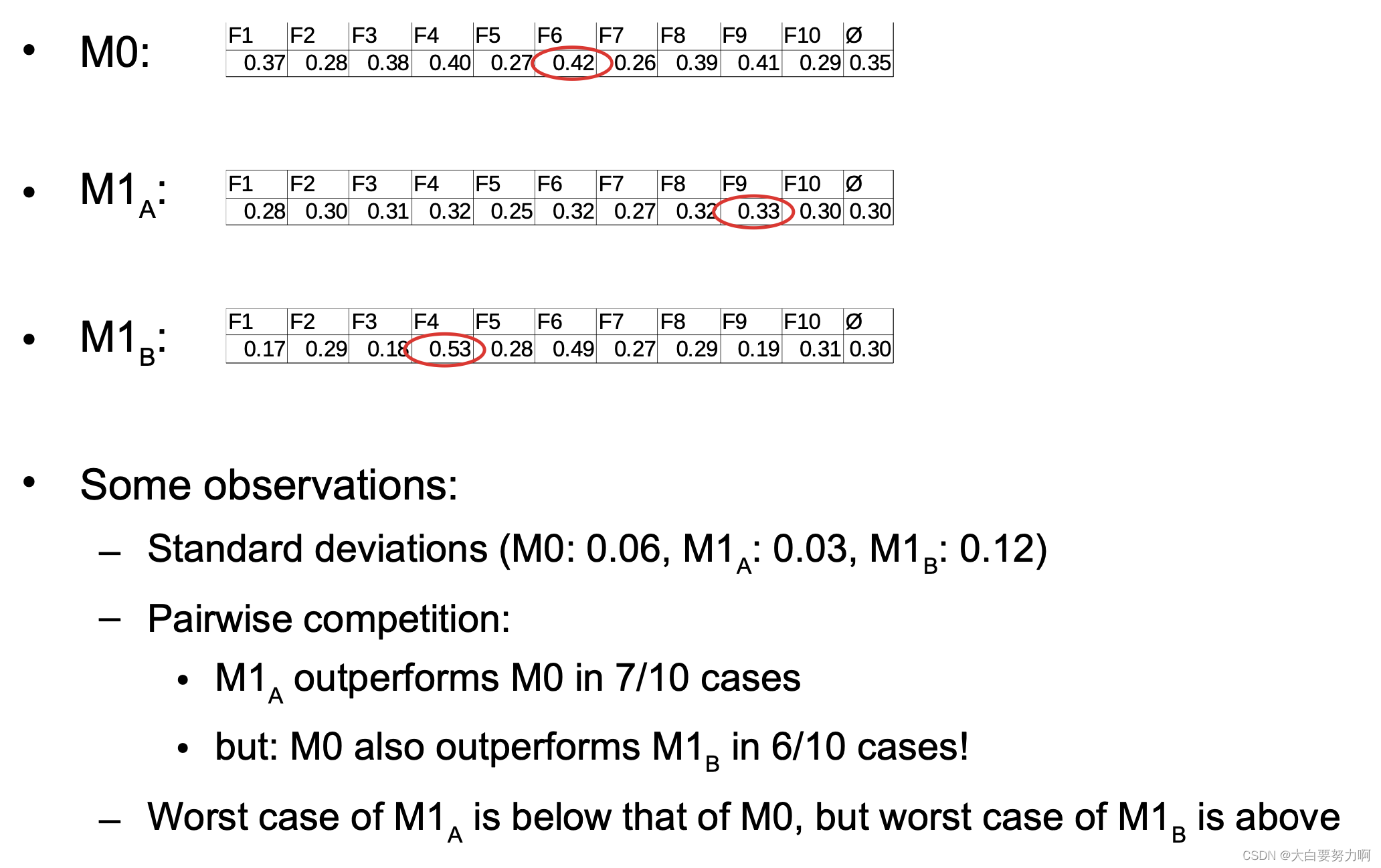
Scenario: you have learned a model M1 with an error rate of 0.30. The old model M0 had an error rate of 0.35 (both evaluated on the same test set T). Do you think the new model is better?

What might be suitable indicators?
Size of the test set, model complexity, model variance

7.3.1 Size of the Test Set

Scenario: you have learned a model M1 with an error rate of 0.30 and the old model M0 had an error rate of 0.35 (both evaluated on the same test set S).

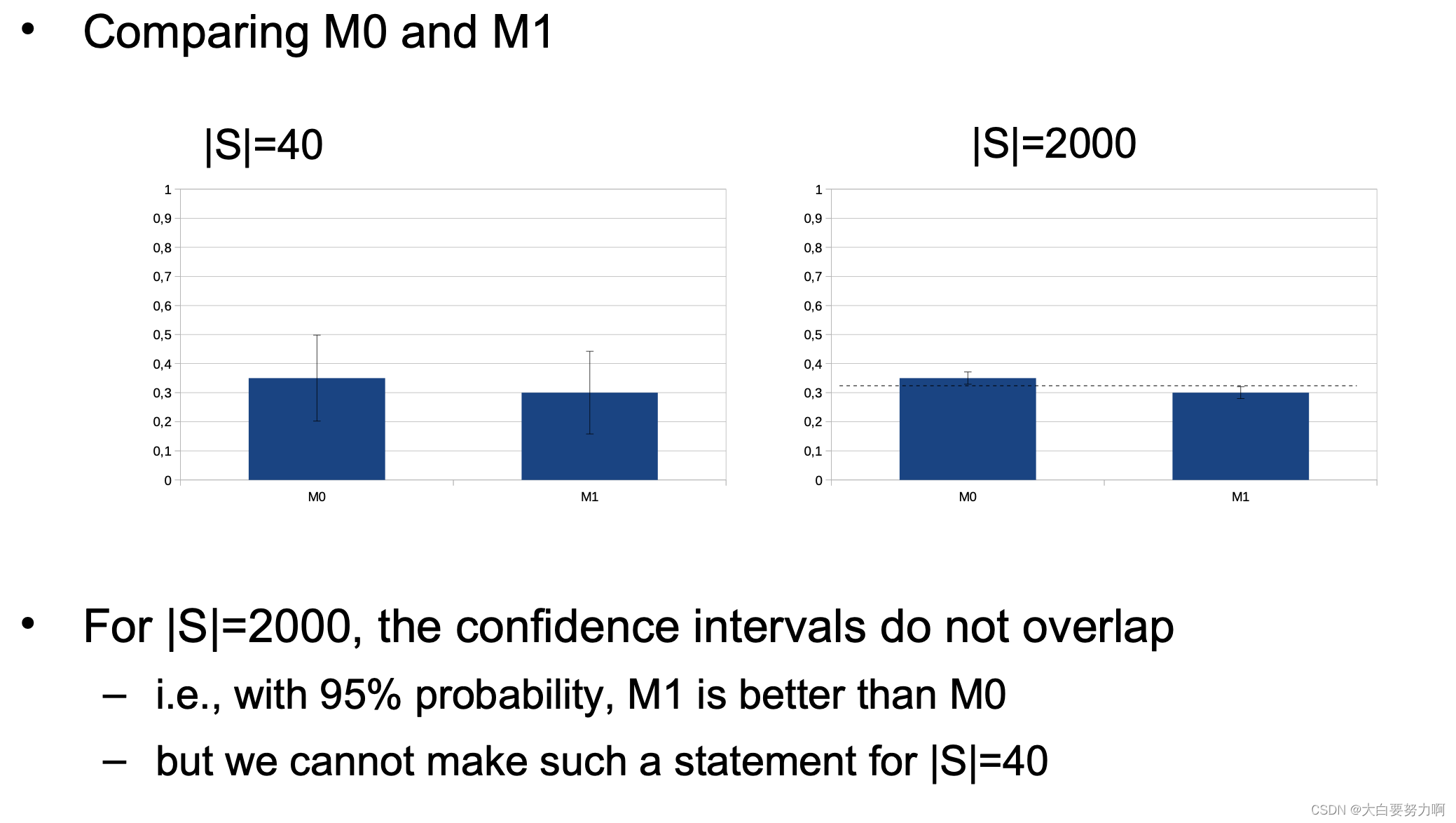
Variant A: |S| = 40
a single error contributes 0.025 to the error rate, i.e., M1 got two more example right than M0

Variant B: |S| = 2,000
a single error contributes 0.0005 to the error rate, i.e., M1 got 100 more examples right than M0

Intuitively:
M1 is better if the error is observed on a larger test set S
The smaller the difference in the error, the larger |S| should be

Most often, the model has overfit to S
Possible reasons: S is a subset of training data (drastic) & S has been used in feature engineering and/or parameter tuning & we have trained and tuned three models only on T, and pick the one which is best on S

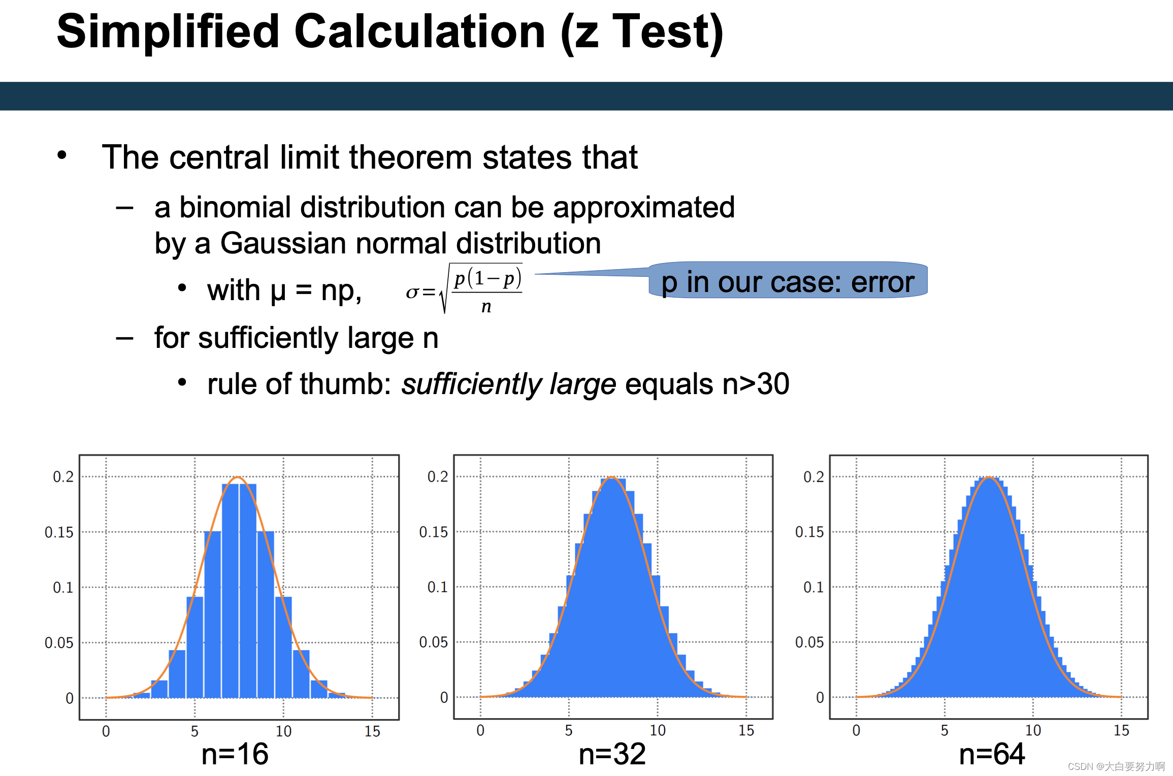
New question: how likely is it the error of M1 is lower just by chance either: due to bias in M1, or due to variance

Consider this a random process:
M1 makes an error on example x
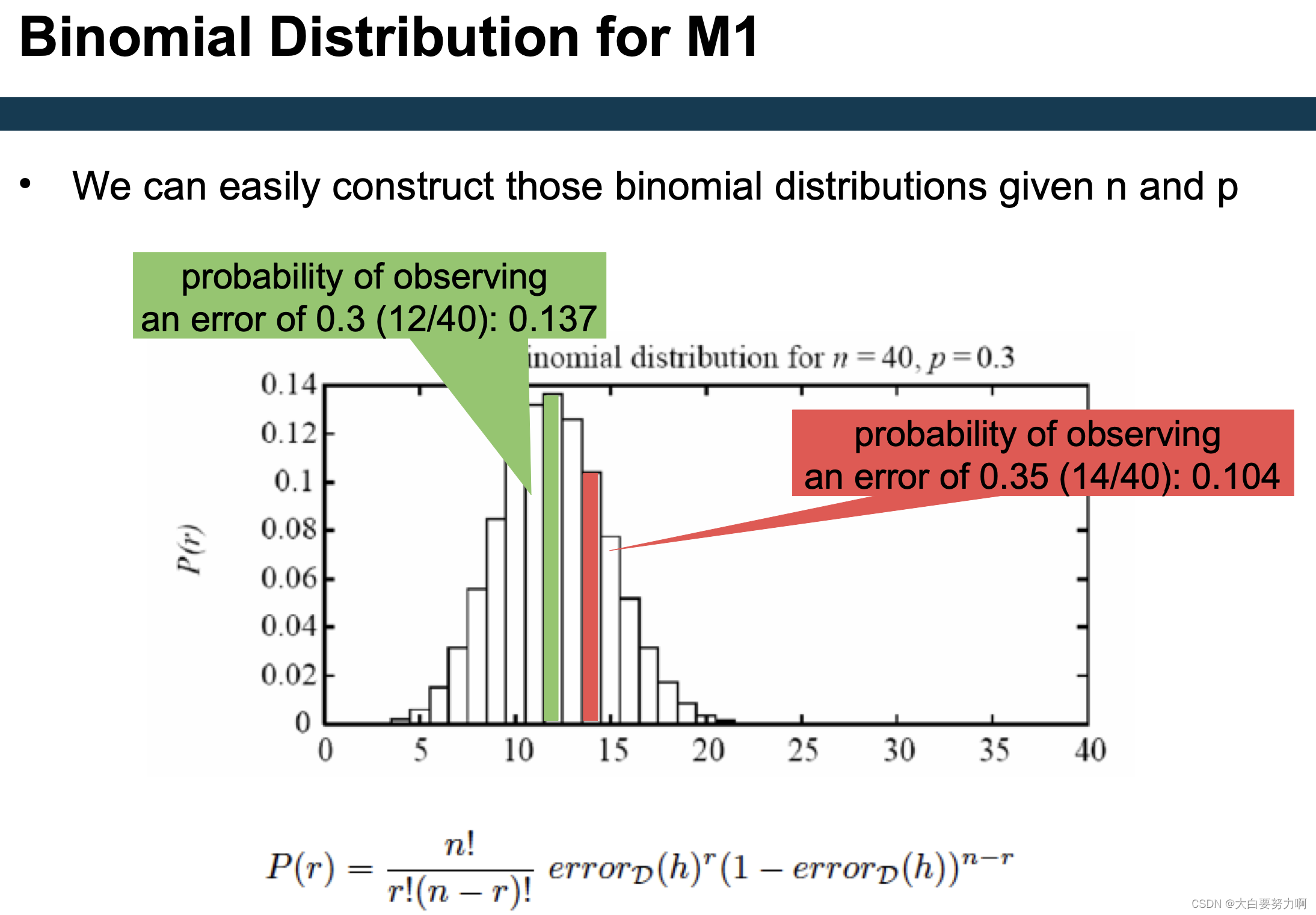
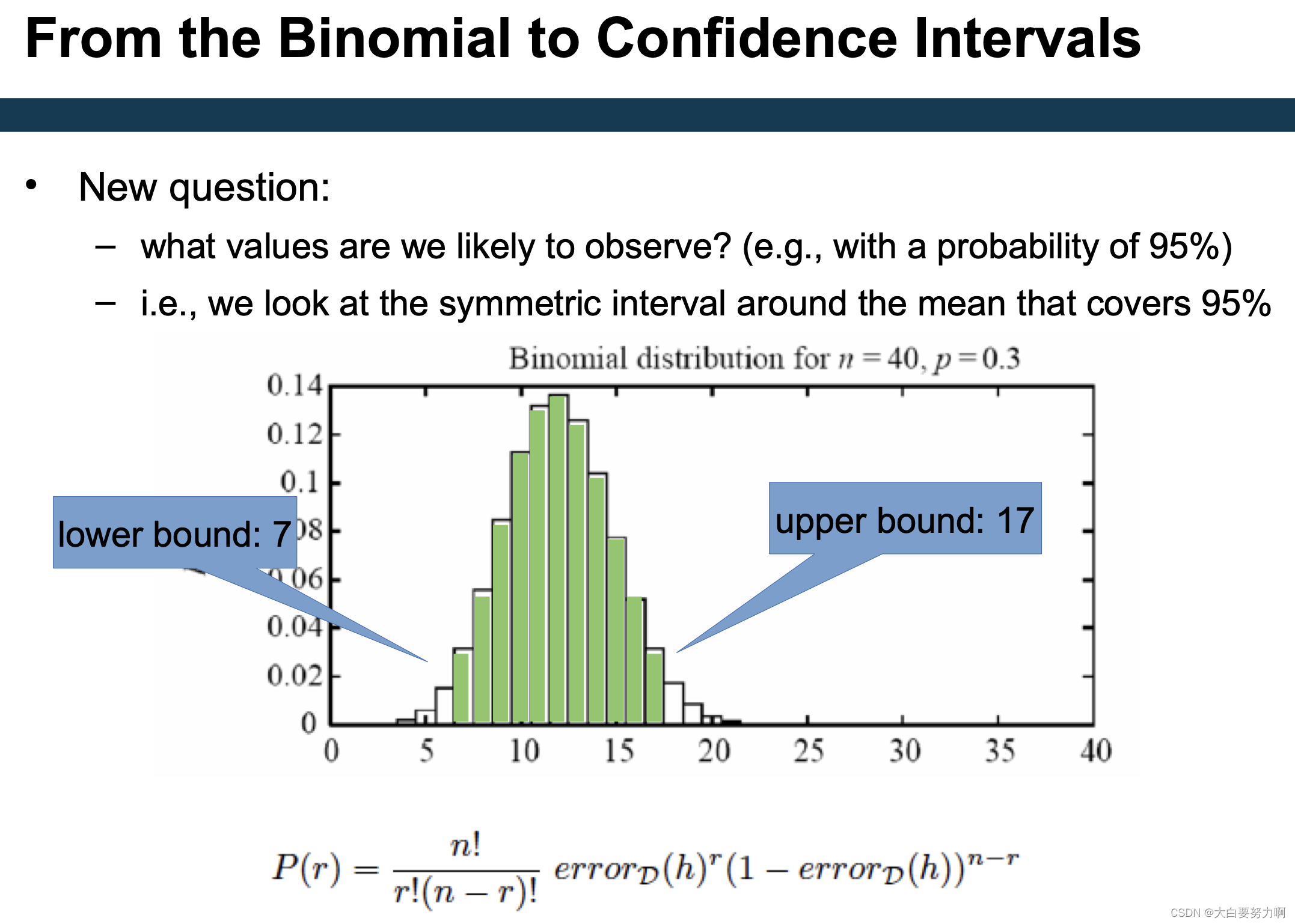
Let us assume it actually has an error rate of 0.3, i.e., M1 follows a binomial with its maximum at 0.3

Test: what is the probability of actually observing 0.3 or 0.35 as error rates?

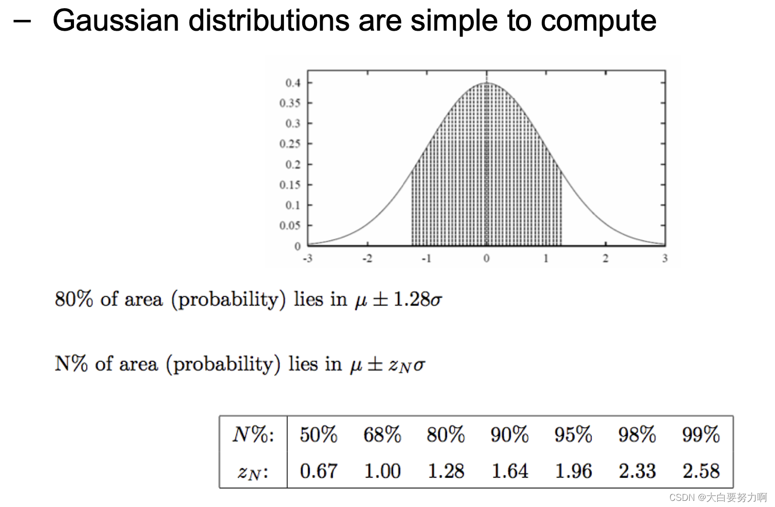
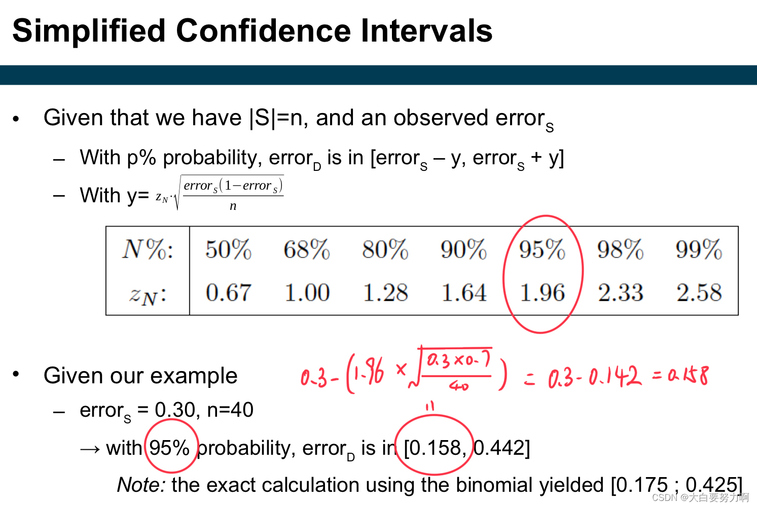
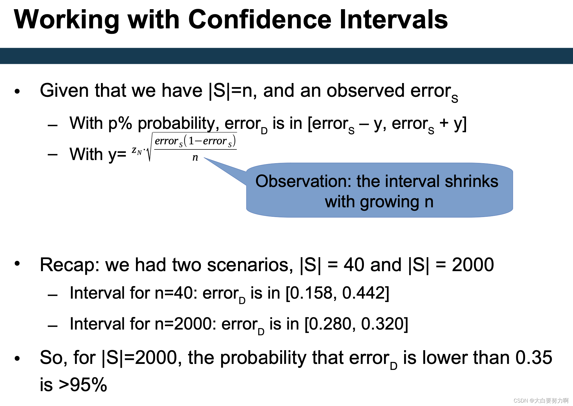
With a probability of 95%, we observe 7 to 17 errors – corresponds to [0.175 ; 0.425] as a confidence interval
All observations in that interval are considered likely – i.e., an observed error rate of 0.35 might also correspond to an actual error rate of 0.3

In our example, on a test sample of |S|=40, we cannot say whether M1 or M0 is better.

7.3.2 Model Complexity

Occam’s Razor
A fundamental principle of science: if you have two theories that explain a phenomenon equally well, choose the simpler one -> if you have two models where none is significantly better than the other, choose the simpler one

Indicators for simplicity: number of features used, number of variables used, e.g., hidden neurons in an ANN, no. of trees in a Random Forest,…

7.3.3 Model Variance

What happens if you repeat an experiment…
– …on a different test set?
– …on a different training set?
– …with a different random seed?

Some methods may have higher variance than others
– if your result was good, was just luck?
– what is your actual estimate for the future?

Typically, we need more than one experiment!

Why is model variance important?
recap: confidence intervals
risk vs. gain (use case!)
often, training data differs
even if you use cross or split validation during development, you might still train a model on the entire training data later

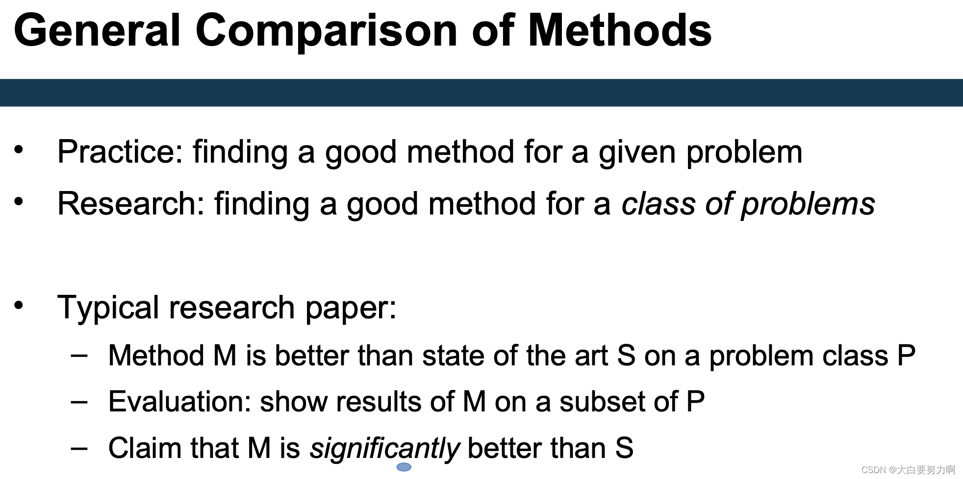
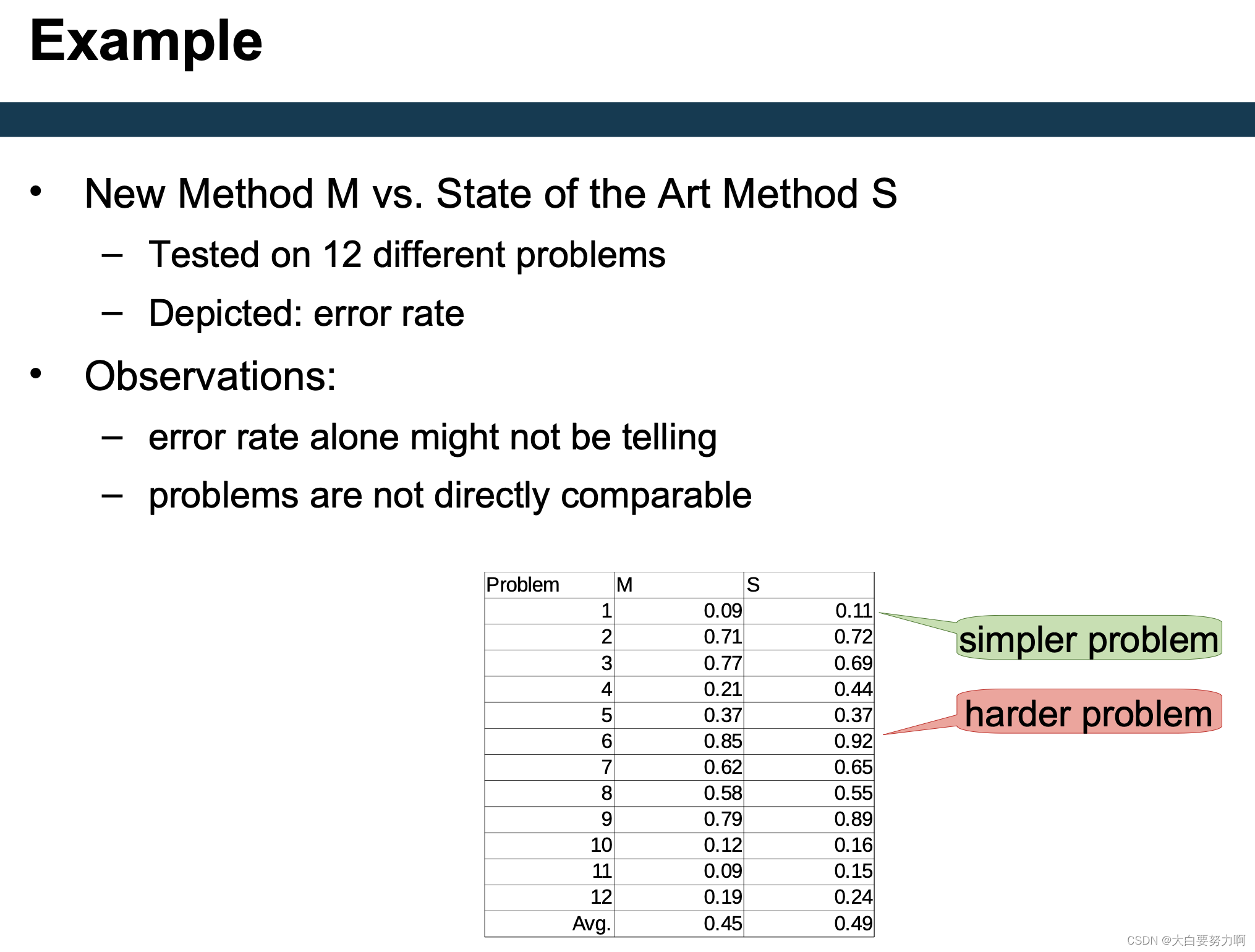
7.4 General Comparison of Methods

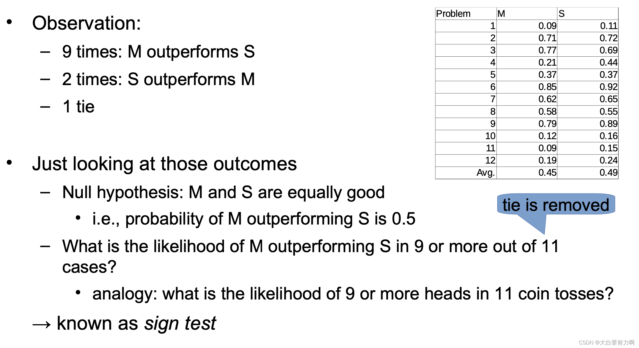
7.5 Sign Test

7.6 Wilcoxon Signed-Rank Test

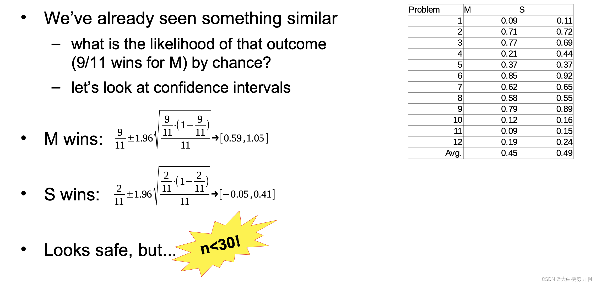
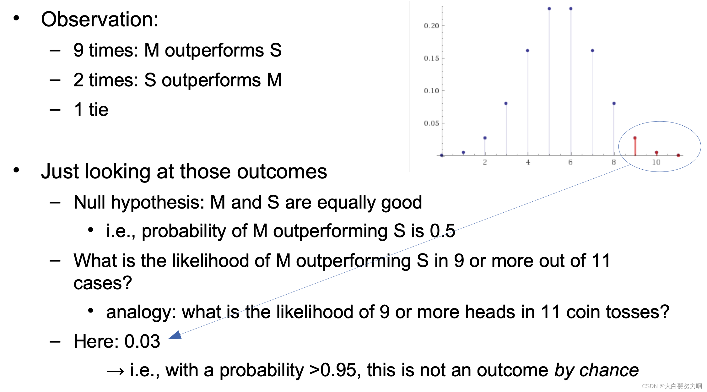
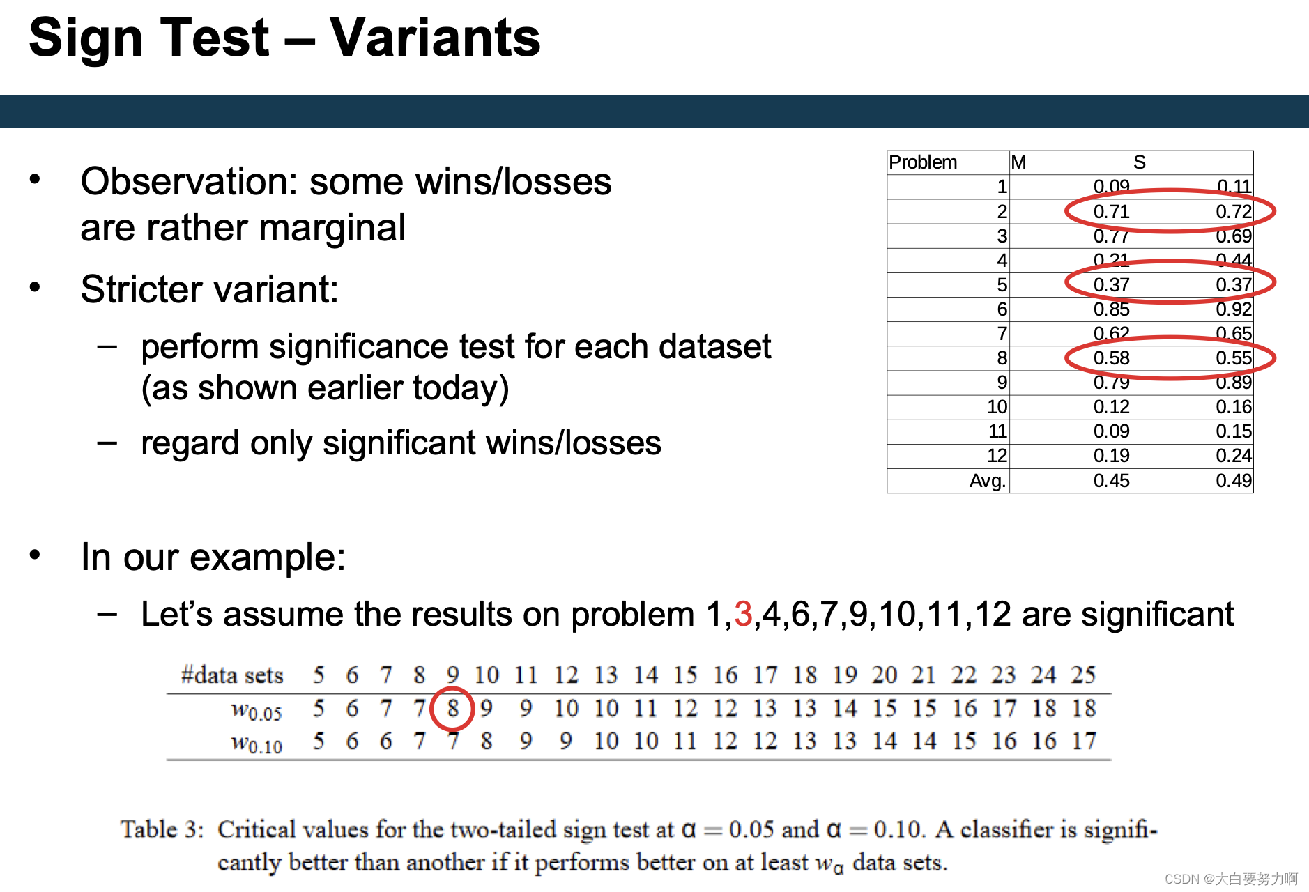
Observation: some wins/losses are rather marginal
Wilcoxon Signed-Rank Test takes margins into account

Approach:

• rank results by absolute difference
• sum up ranks for positive and negative outcomes
  • best case: all outcomes positive → sum of negative ranks = 0
  • still good case: all negative outcomes are marginal → sum of negative ranks is low

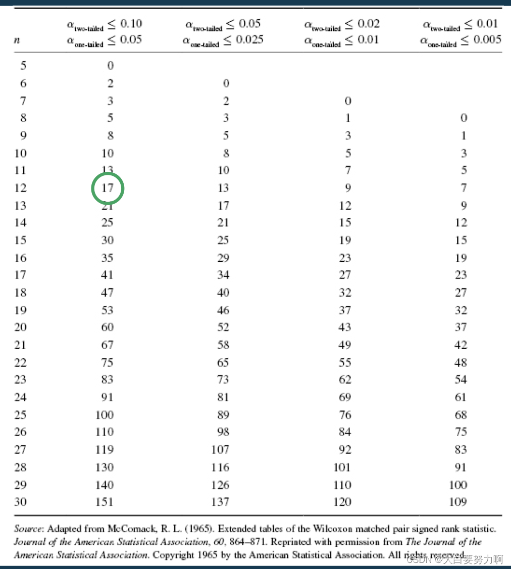
We use the one-tailed test because we want to test if M is better than S
14.5 < 17 → the results are significant

Tests for Comparing Approaches Summary

1. Simple z test only reliable for many datasets (>30)
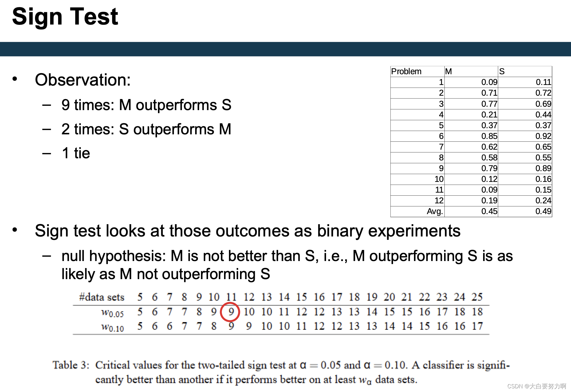
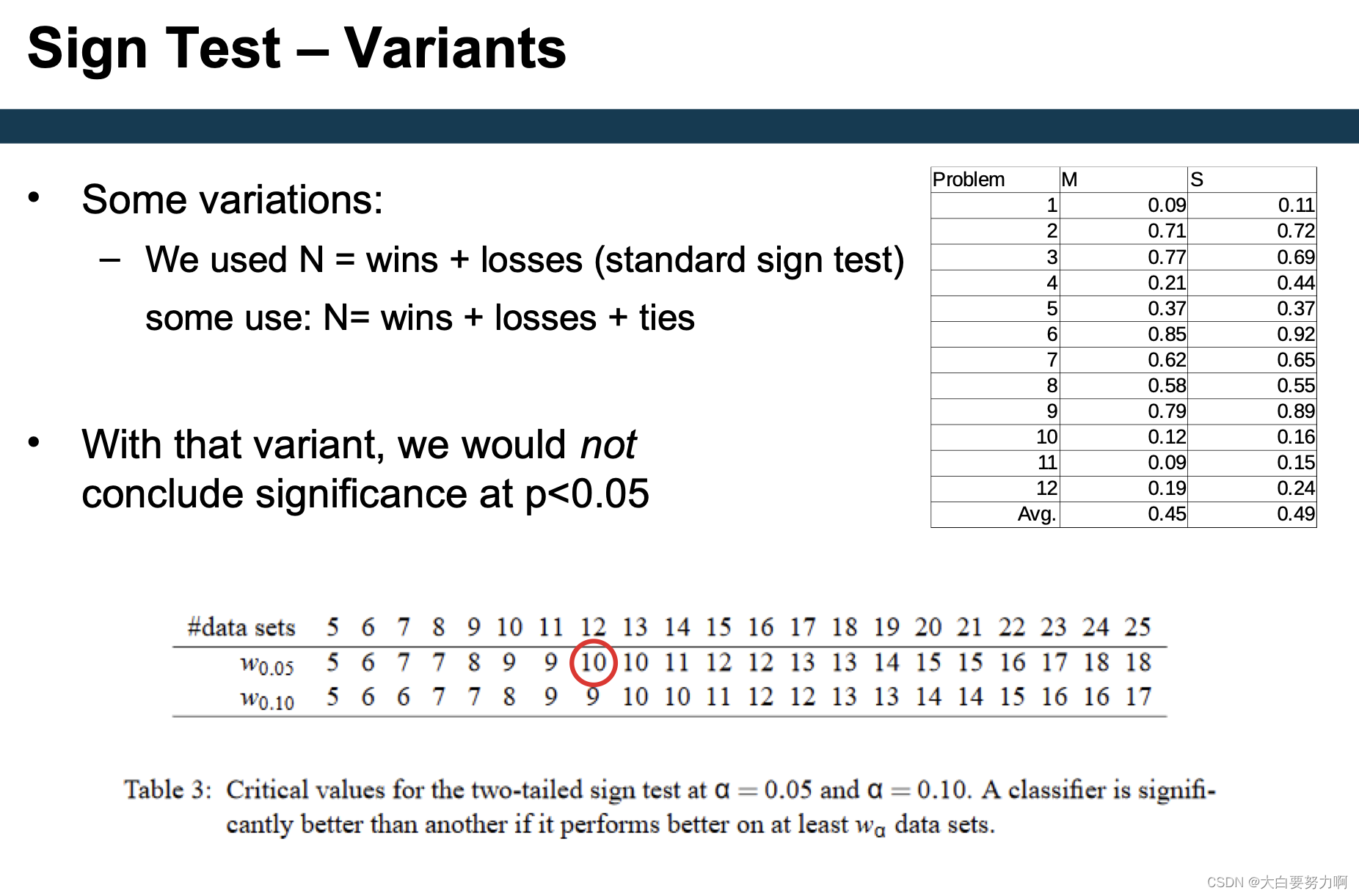
2. Sign test does not distinguish large and small margins
3. Wilcoxon signed-rank test - works also for small samples (e.g., half a dozen datasets) and considers large and small margins

7.7 Ablation Studies

Often, data mining pipelines are complex. Different preprocessing approaches, adding external data, computing extra features, …

Each of those steps may be left out or replaced by a simpler baseline.
This is called an ablation study.
i.e., does that change bear a significant advantage? – recap: Occam’s razor!

7.7.1 Measuring Model Simplicity

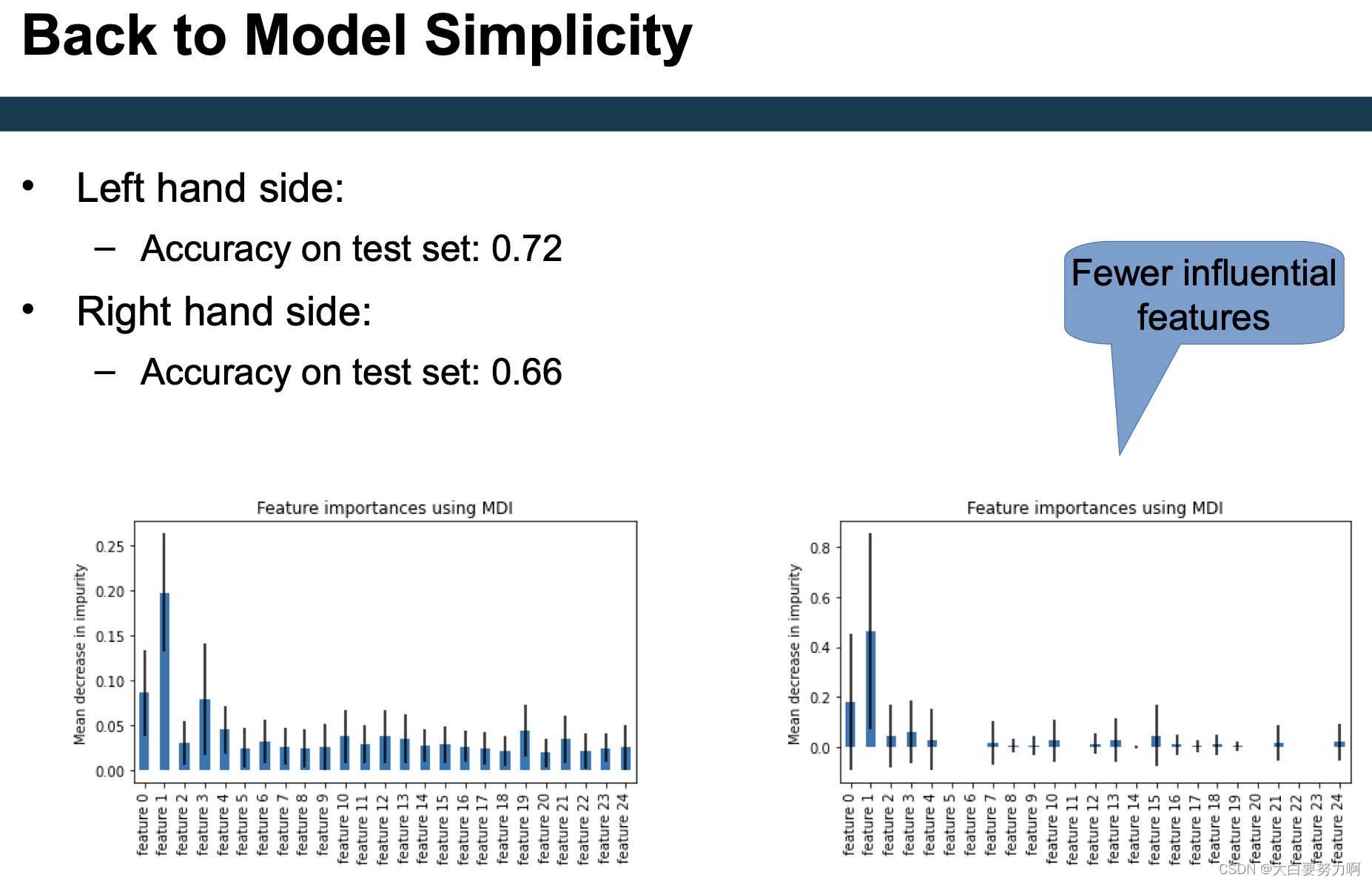
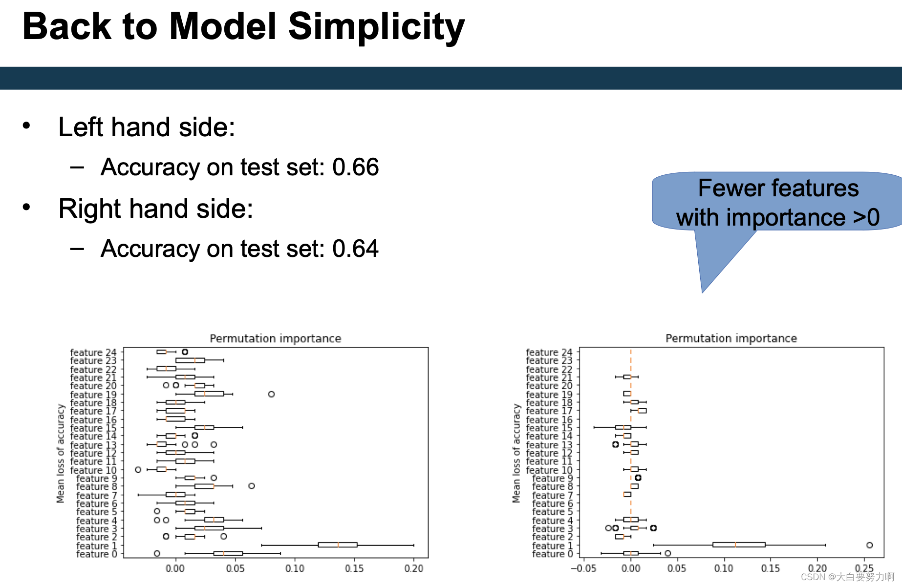
Idea: the less feature the model focuses on, the simpler
Not necessarily: the better (Caveats: identifiers, false predictors, …)

Good models have both low test error and low complexity

7.7.2 Measuring Feature Importance

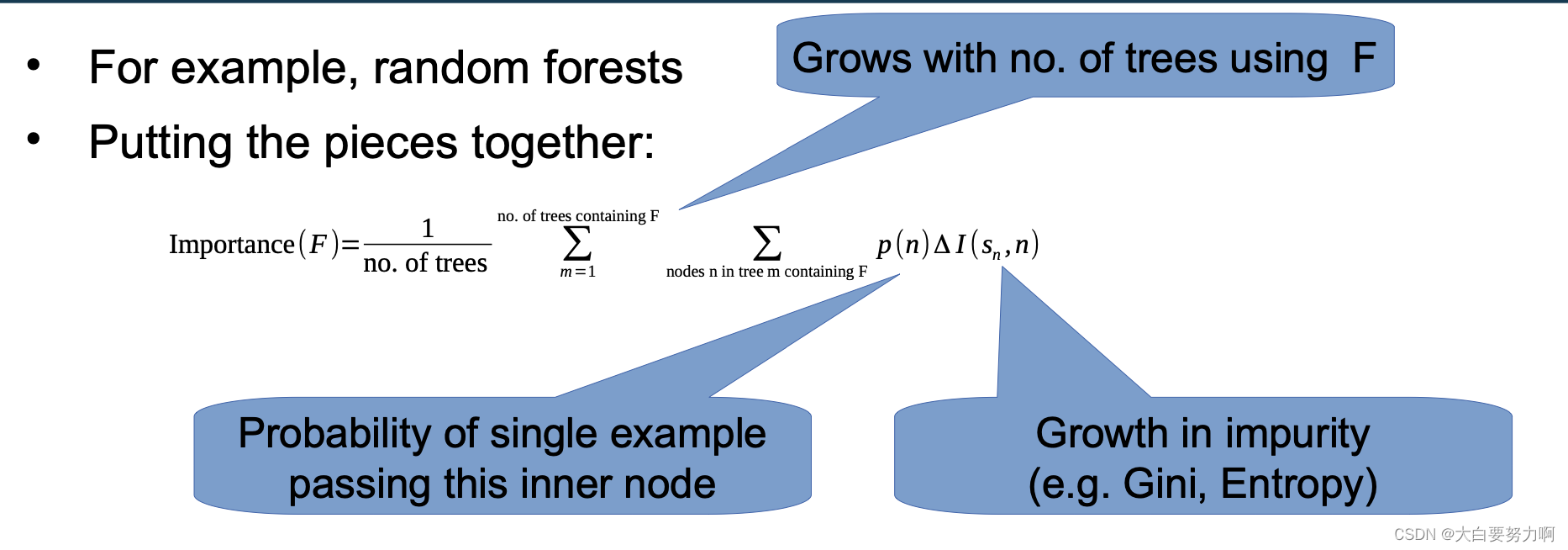
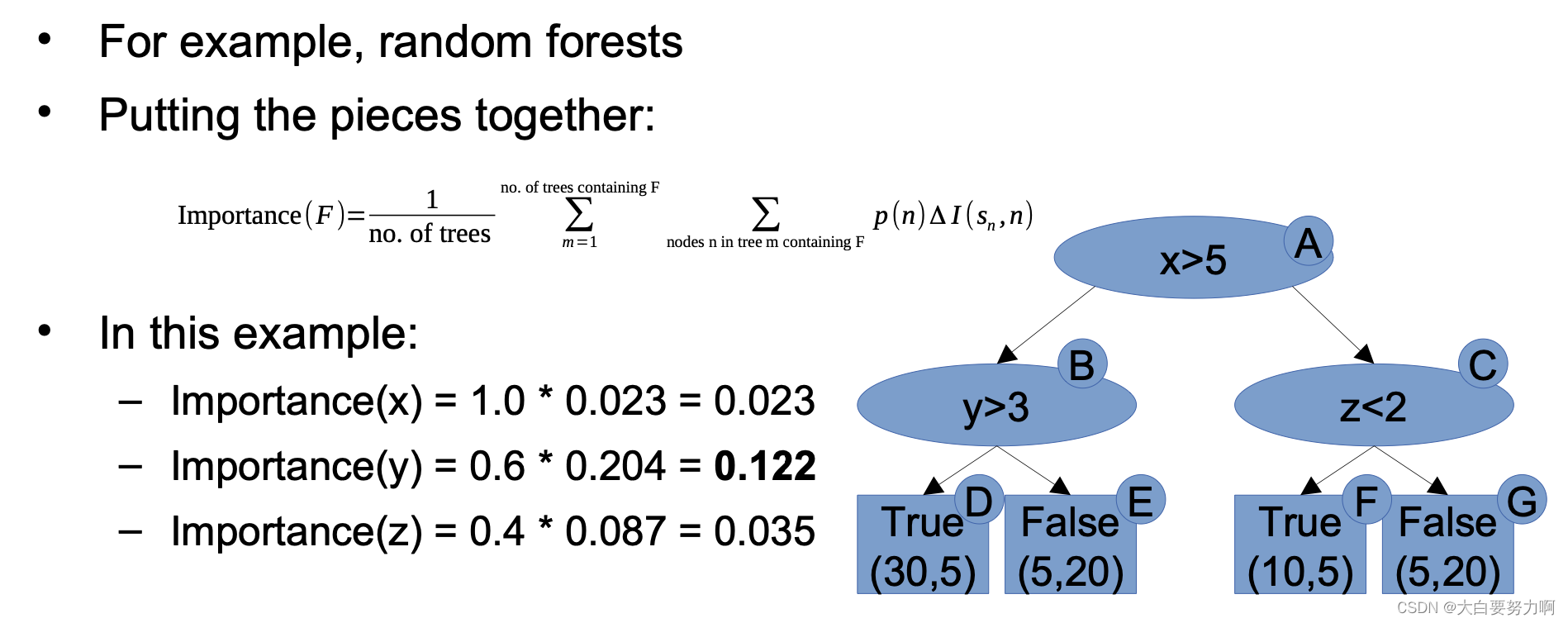
Example: random forests
A feature is more important if
(1) it is used in many trees
Rationale: weighted prediction across trees. The more trees it is used in, the higher the influence
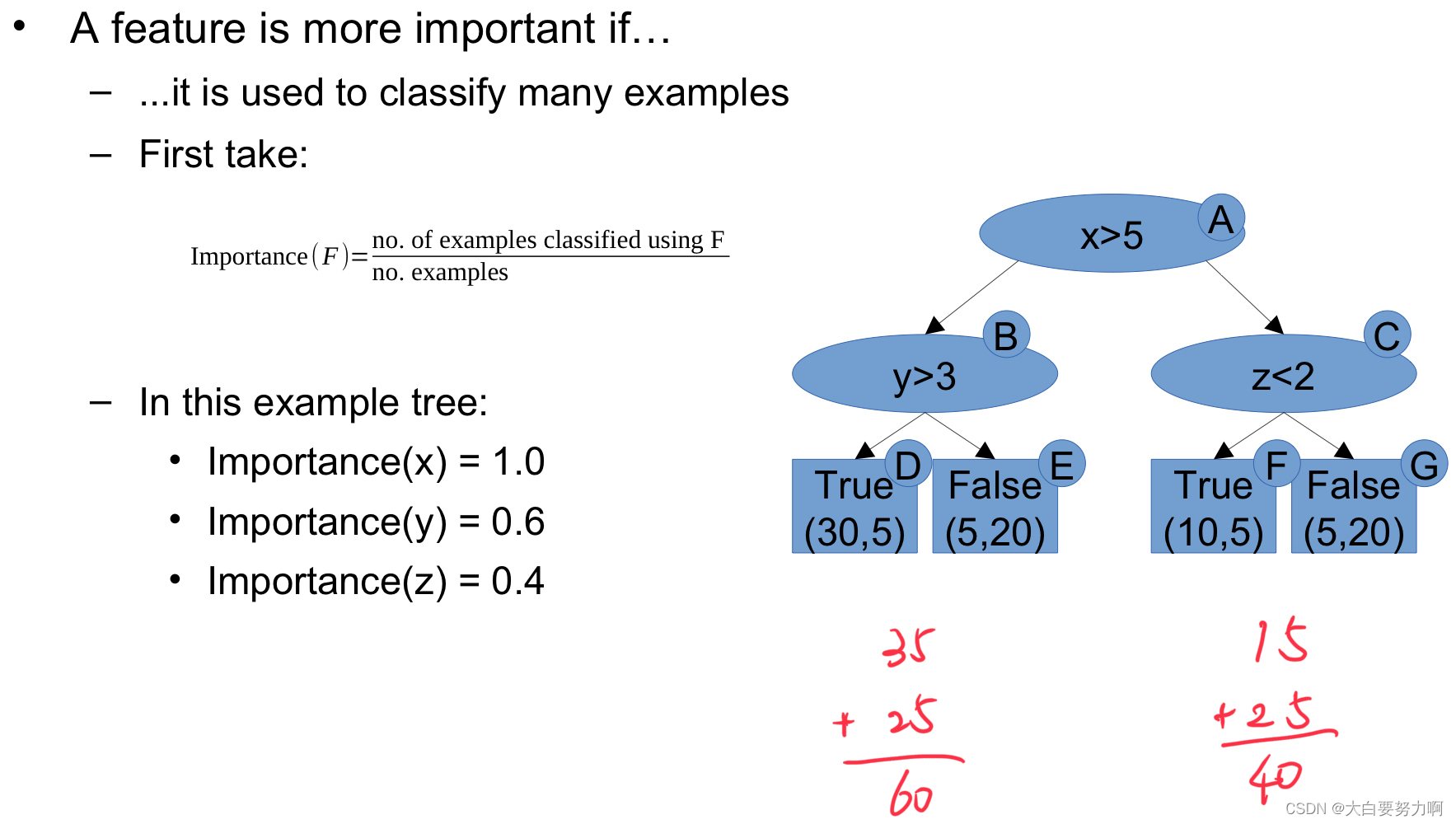
(2) it is used to classify many examples
Rationale: more predictions are influenced by that attribute, i.e., for a single example: higher likelihood of influence
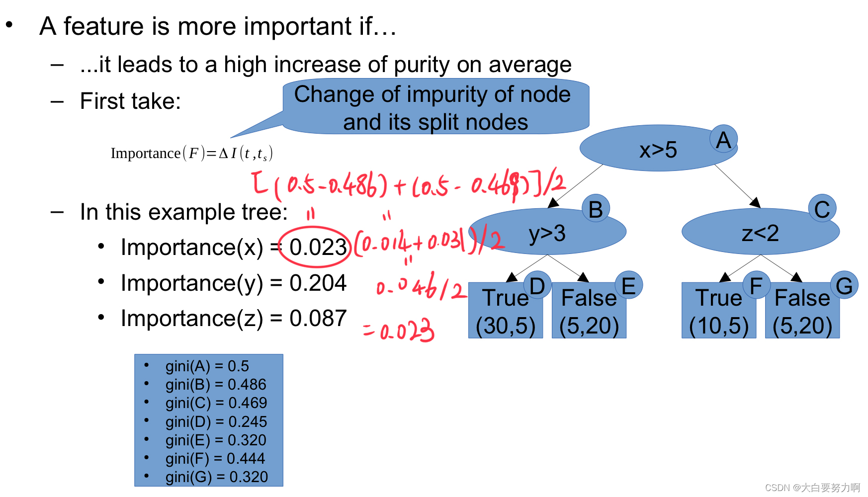
(3) it leads to a high increase of purity on average
Rationale: if the purity is not increased, the split is rather a toin coss

Feature Weights and Model Simplicity
If you have two models where none is significantly better than the other, choose the simpler one.

Feature weights
Can indicate model simplicity (few high weighted features)

Examples for computation
Random Forest, XGBoost: Mean Decrease in Impurity (MDI)
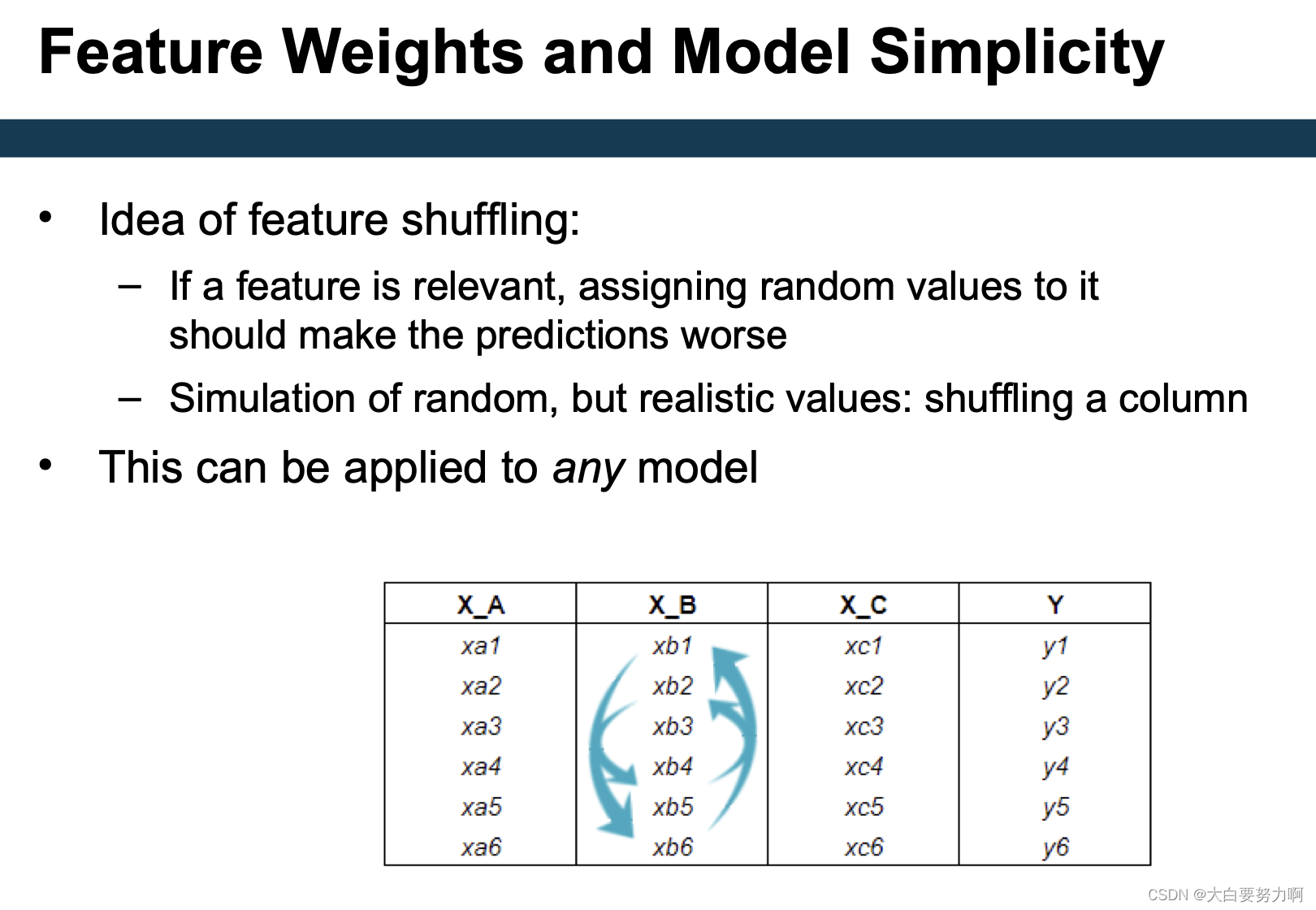
General: feature shuffling

7.7 LIME Model Explanation

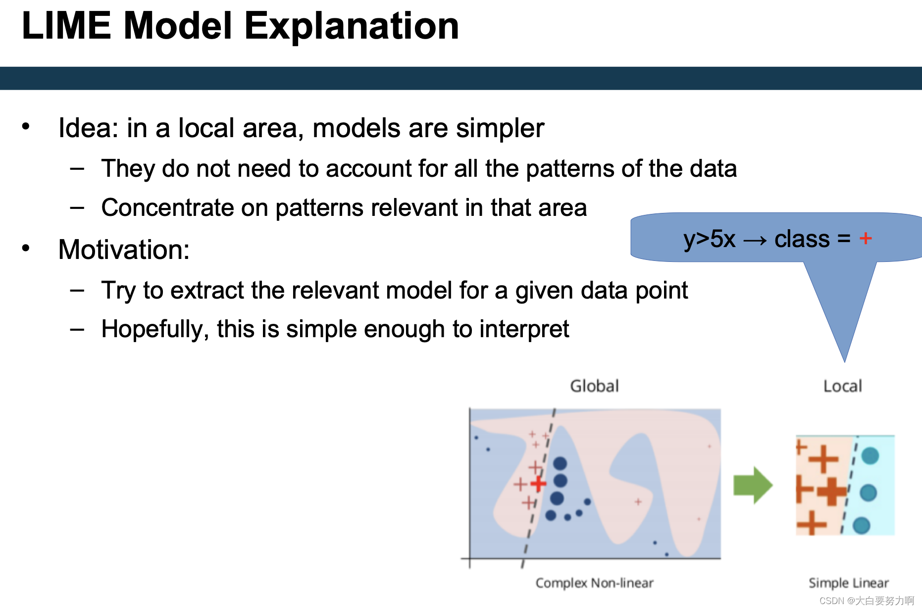
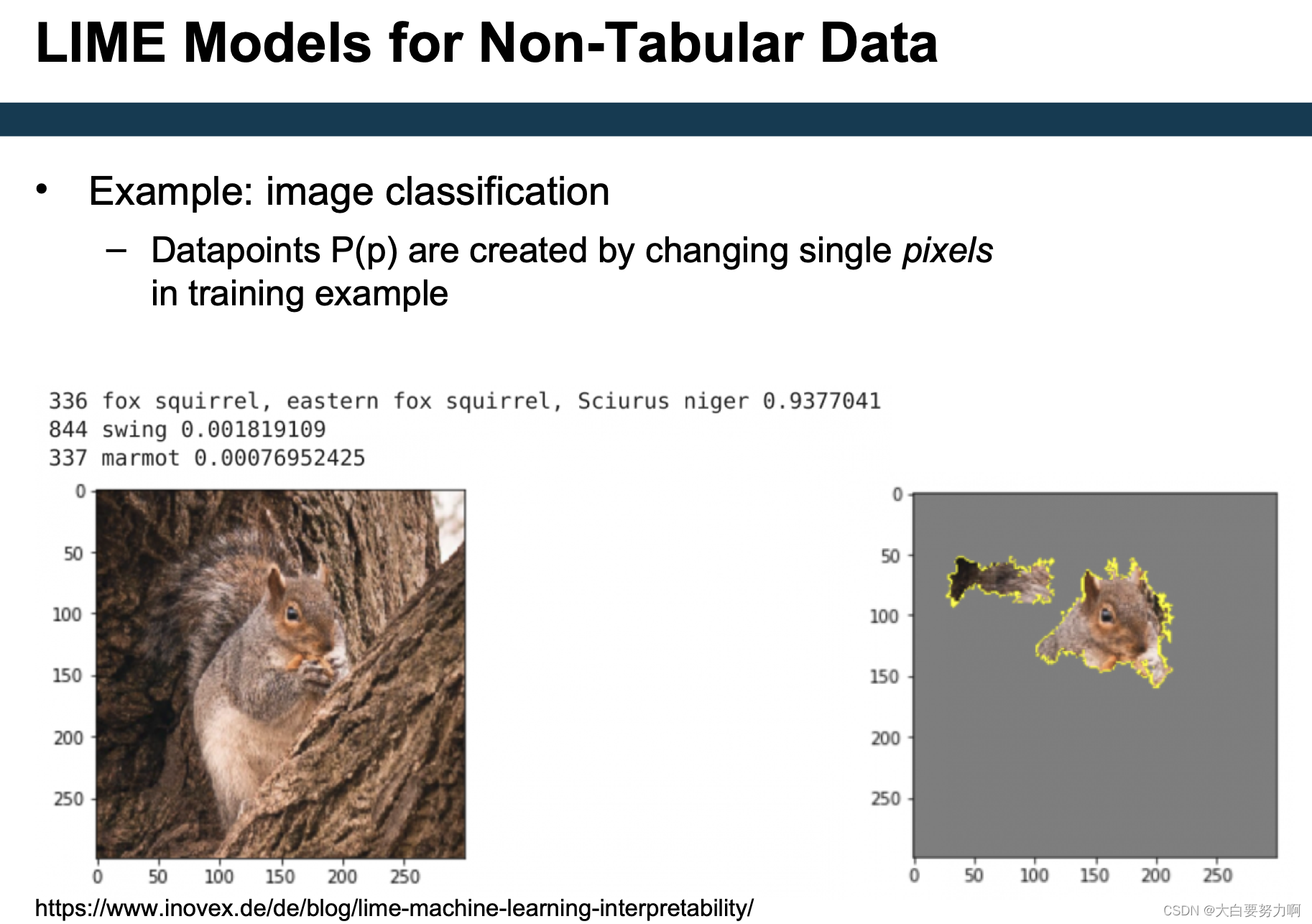
How to interpret a “black box” (i.e., uninterpretable) model M?
Local: for a datapoint p
Basic idea:

1. create artificial datapoints P(p) in vicinity of p
2. score each p’ in P with black box model
3. learn interpretable model M’ → values: P, labels: scores of M
4. create prediction for p using M’ or analyze M’ directly

Results in Data Mining are often reduced to a single number, e.g., accuracy, error rate, F1, RMSE. Result differences are often marginal

Problem of unseen data: we can only guess/approximate the true performance on unseen data, which makes it hard to select between approaches

Helpful tools: confidence intervals, significance tests, and Occam’sRazor

Model inspection on global level:

• Model complexity
• Proxy:feature importance
• Less complex model → more likely to generalize

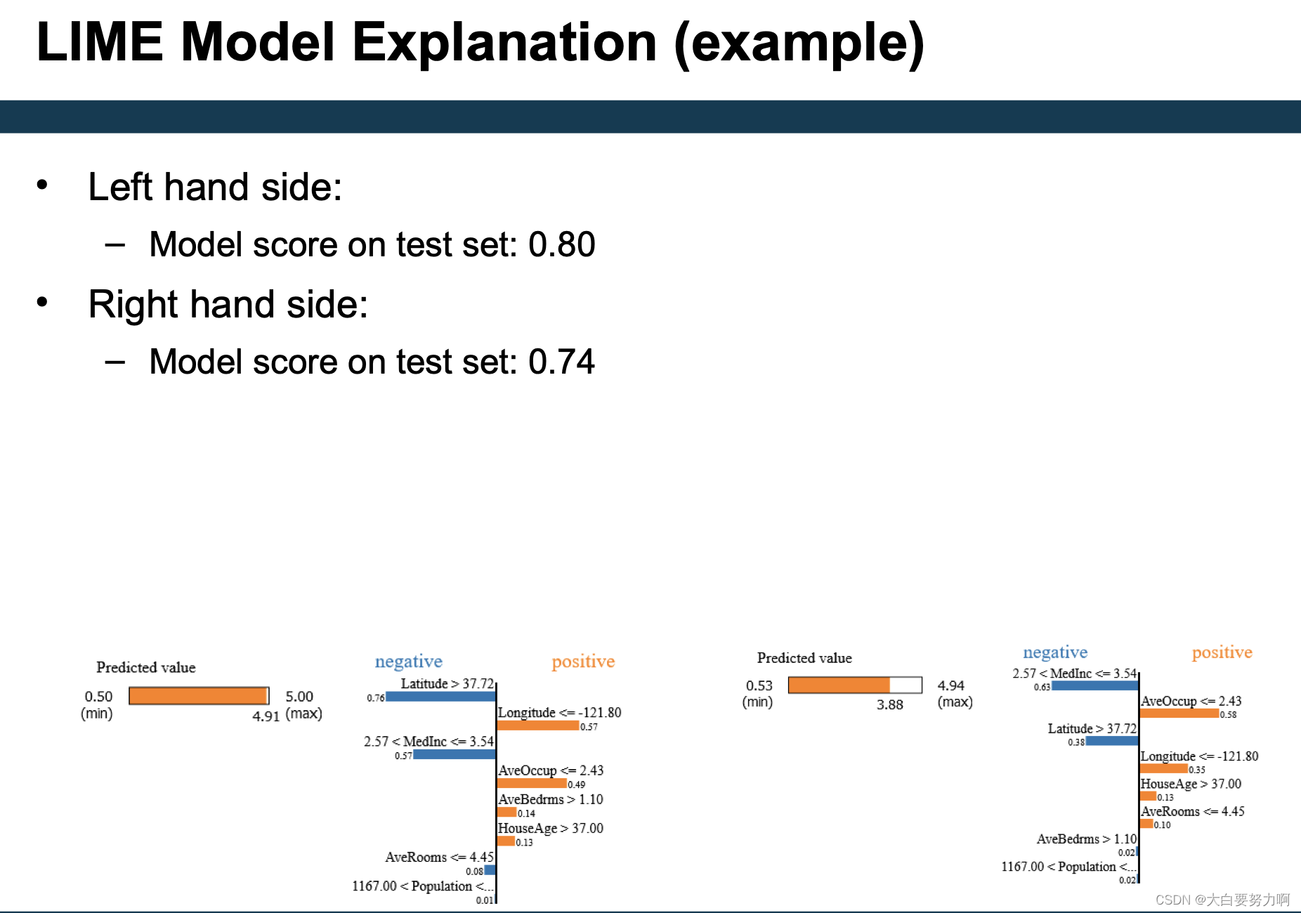
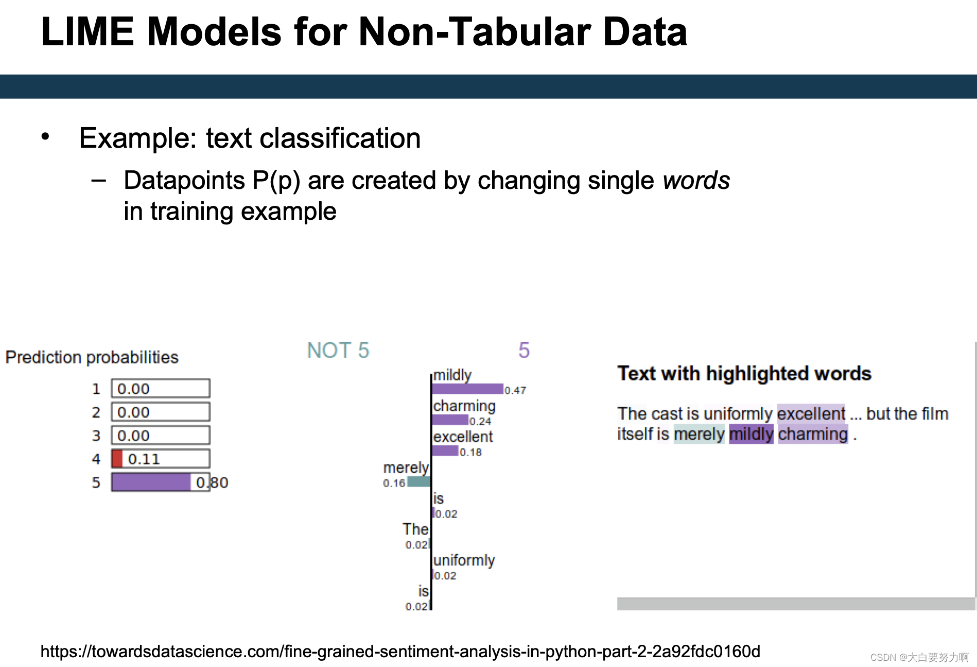
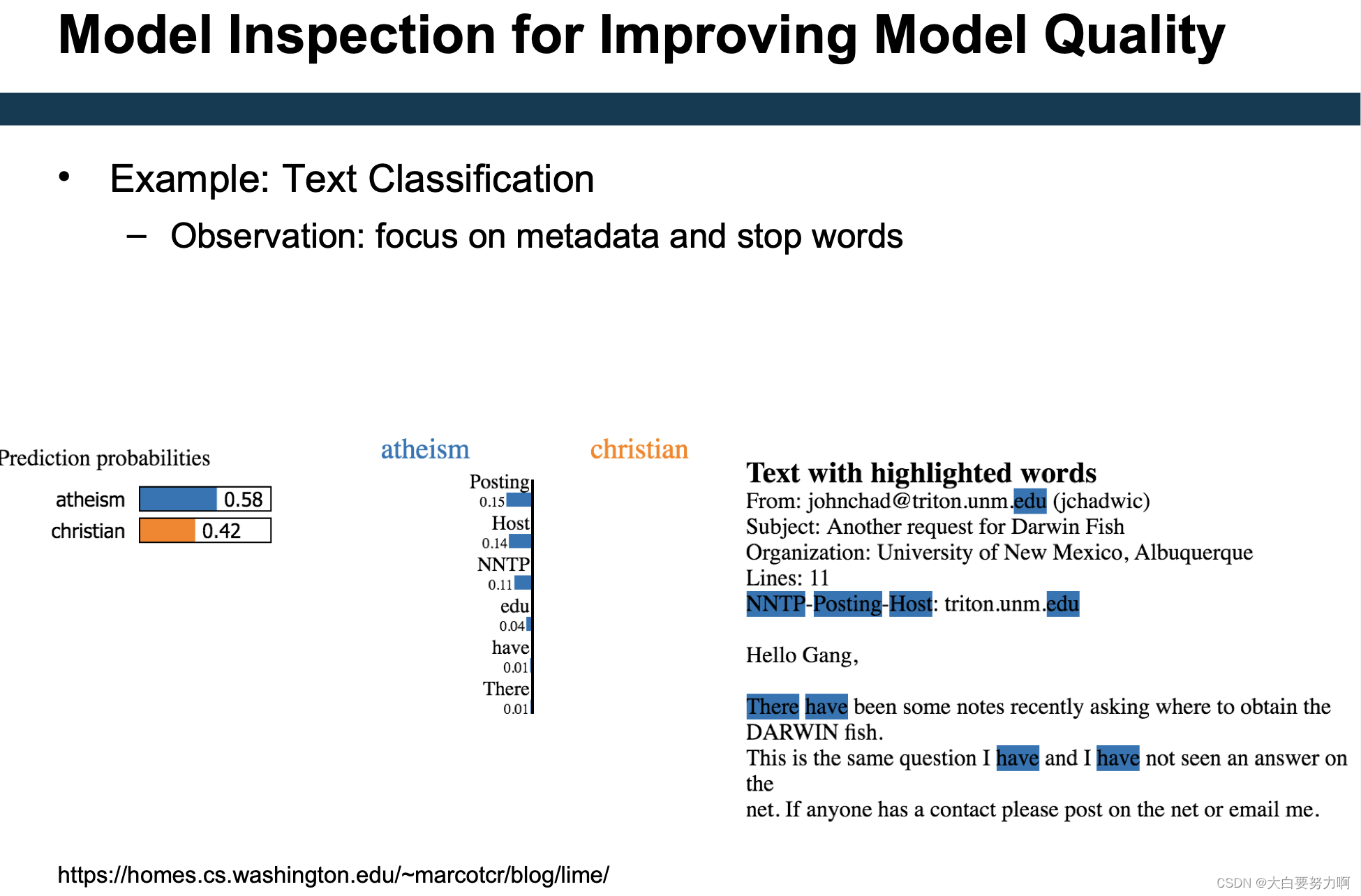
Model inspection on local level

• Generating explanations for test instances
• Do they look plausible?