论文地址:VoxelNet: End-to-End Learning for Point Cloud Based 3D Object Detection
代码地址:https://github.com/Hqss/VoxelNet_PyTorch
一、引言
VoxelNet不同于之前的pointxet直接对原始点云进行特征提取的方案,提出了将点云体素化(网格化)的提取方案,极大地提高了点云网络的计算效率,具体流程如图1所示。

具体步骤:
(1)首先对原始激光点云进行体素化处理,构建一个个小栅格,包围整个点云,并对每一个体素栅格进行编码。
(2)遍历原始点云,给每个点云中的点分配一个体素栅格索引,也就是找到每一个栅格中包含哪些点云,再对每一个栅格中随机采样T个点作为该栅格的点云特征(保证了每一个体素块中点云数目是均匀的)。
(3)使用特征编码网络Feature Encoding对(2)构建的voxel体素特征进行特征提取。
(4)使用RPN网络对Feature Encoding的输出特征进行映射,得到cls的置信度分数和回归框bounding box大小。
二、pipeline
2.1 VoxelNet网络结构
2.1.1 aug_data 点云数据增强
2.1.1.1 原理:
VoxelNet选择的是随机点云数据增强方案,随机生成一个0~10之间的数,根据生成数的大小来选择点云数据增强方式,有点云旋转、点云缩放等。
注:这里的点云数据增强比较类似图像数据增强,包括旋转、缩放等,这里建议取仔细阅读一下代码,比较杂。
2.1.1.2 代码:
def aug_data(tag, object_dir):
    # 数据增强的函数 aug_data(tag, object_dir),用于处理点云数据和图像数据,增加数据的多样性以提升模型的鲁棒性和泛化能力。
    np.random.seed()

    # rgb = cv2.imread(os.path.join(object_dir,'image_2', tag + '.png'))
    rgb = cv2.resize(cv2.imread(os.path.join(object_dir, 'image_2', tag + '.png')), (cfg.IMAGE_WIDTH, cfg.IMAGE_HEIGHT))
    lidar = np.fromfile(os.path.join(object_dir, 'velodyne', tag + '.bin'), dtype = np.float32).reshape(-1, 4)
    label = np.array([line for line in open(os.path.join(object_dir, 'label_2', tag + '.txt'), 'r').readlines()])  # (N')

    cls = np.array([line.split()[0] for line in label])  # (N')
    gt_box3d = label_to_gt_box3d(np.array(label)[np.newaxis, :], cls = '', coordinate = 'camera')[0]  # (N', 7); 7 means (x, y, z, h, w, l, r)

    # 选择数据增强方式:
    # 通过随机数 choice 的值来决定采用哪种数据增强方式:
    # choice >= 7:禁用某些增强方法。
    # choice < 7 and choice >= 4:进行全局旋转操作。
    # choice < 4:进行全局缩放操作。
    choice = np.random.randint(0, 10)
    if choice >= 7:
        # Disable this augmention here. Current implementation will decrease the performances.

        lidar_center_gt_box3d = camera_to_lidar_box(gt_box3d)

        lidar_corner_gt_box3d = center_to_corner_box3d(lidar_center_gt_box3d, coordinate = 'lidar')

        for idx in range(len(lidar_corner_gt_box3d)):
            # TODO: precisely gather the point
            is_collision = True
            _count = 0
            while is_collision and _count < 100:
                t_rz = np.random.uniform(-np.pi / 10, np.pi / 10)
                t_x = np.random.normal()
                t_y = np.random.normal()
                t_z = np.random.normal()

                # Check collision
                tmp = box_transform(lidar_center_gt_box3d[[idx]], t_x, t_y, t_z, t_rz, 'lidar')
                is_collision = False
                for idy in range(idx):
                    x1, y1, w1, l1, r1 = tmp[0][[0, 1, 4, 5, 6]]
                    x2, y2, w2, l2, r2 = lidar_center_gt_box3d[idy][[0, 1, 4, 5, 6]]
                    iou = cal_iou2d(np.array([x1, y1, w1, l1, r1], dtype = np.float32),np.array([x2, y2, w2, l2, r2], dtype = np.float32))
                    if iou > 0:
                        is_collision = True
                        _count += 1
                        break

            if not is_collision:
                box_corner = lidar_corner_gt_box3d[idx]
                minx = np.min(box_corner[:, 0])
                miny = np.min(box_corner[:, 1])
                minz = np.min(box_corner[:, 2])
                maxx = np.max(box_corner[:, 0])
                maxy = np.max(box_corner[:, 1])
                maxz = np.max(box_corner[:, 2])
                bound_x = np.logical_and(lidar[:, 0] >= minx, lidar[:, 0] <= maxx)
                bound_y = np.logical_and(lidar[:, 1] >= miny, lidar[:, 1] <= maxy)
                bound_z = np.logical_and(lidar[:, 2] >= minz, lidar[:, 2] <= maxz)
                bound_box = np.logical_and(np.logical_and(bound_x, bound_y), bound_z)
                lidar[bound_box, 0:3] = point_transform(lidar[bound_box, 0:3], t_x, t_y, t_z, rz = t_rz)
                lidar_center_gt_box3d[idx] = box_transform(lidar_center_gt_box3d[[idx]], t_x, t_y, t_z, t_rz, 'lidar')

        gt_box3d = lidar_to_camera_box(lidar_center_gt_box3d)
        newtag = 'aug_{}_1_{}'.format(tag, np.random.randint(1, 1024))


    elif choice < 7 and choice >= 4:
        # Global rotation 全局旋转
        angle = np.random.uniform(-np.pi / 4, np.pi / 4)
        lidar[:, 0:3] = point_transform(lidar[:, 0:3], 0, 0, 0, rz = angle)
        lidar_center_gt_box3d = camera_to_lidar_box(gt_box3d)
        lidar_center_gt_box3d = box_transform(lidar_center_gt_box3d, 0, 0, 0, r = angle, coordinate = 'lidar')
        gt_box3d = lidar_to_camera_box(lidar_center_gt_box3d)
        newtag = 'aug_{}_2_{:.4f}'.format(tag, angle).replace('.', '_')

    else:
        # Global scaling 全局缩放
        factor = np.random.uniform(0.95, 1.05)                       #
        lidar[:, 0:3] = lidar[:, 0:3] * factor                                 # 对点云xyz坐标进行缩放
        lidar_center_gt_box3d = camera_to_lidar_box(gt_box3d)                  #
        lidar_center_gt_box3d[:, 0:6] = lidar_center_gt_box3d[:, 0:6] * factor #
        gt_box3d = lidar_to_camera_box(lidar_center_gt_box3d)                  #
        newtag = 'aug_{}_3_{:.4f}'.format(tag, factor).replace('.', '_')

    label = box3d_to_label(gt_box3d[np.newaxis, ...], cls[np.newaxis, ...], coordinate = 'camera')[0]  # (N')

    voxel_dict = process_pointcloud(lidar)  # 点云体素化函数

    return newtag, rgb, lidar, voxel_dict, label
2.1.2 Voxel Partition 点云体素化(process_pointcloud)
2.1.2.1 原理:
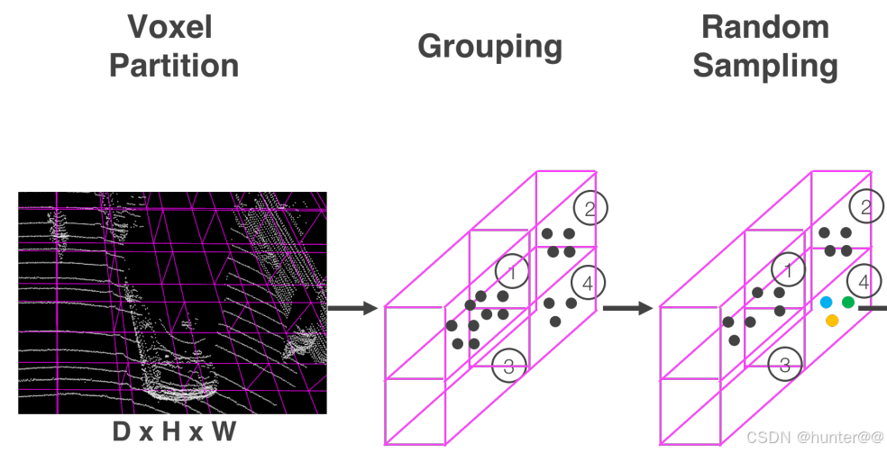
Voxel Partition体素化是Voxelnet最为关键的一步,也是其区别与其他点云处理网络的重点,这里其实也可以理解为是对原始点云的预处理工作。这中间主要包含三步:Voxel Partition、Grouping、Random Sampling。
(1)Voxel Partition的作用是将3D空间中的点云细分为一个一个等间隔的体素,如图2最左侧所示。通过定义每一个体素的大小为

代码中是通过 voxel_index = np.floor(shifted_coord[:, ::-1] / voxel_size).astype(np.int)函数来实现的,这里的 shifted_coord[:, ::-1] 是将xyz进行逆序排列,也就是(X, Y, Z) -> (Z, Y, X),因为论文中设定的voxel_size是按照(Z, Y, X)来排列的。
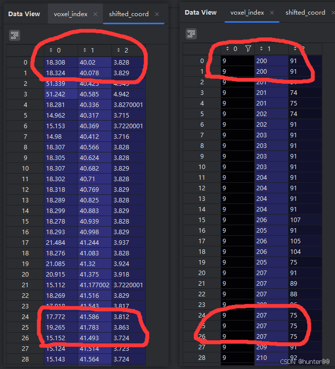
这里的int取整操作才是体素化的核心,因为我们的原始点云都是一堆float32类型的变量,除以voxel_size之后还是float32的变量,这样的体素化是没有意义的;举一个例子来说,就比如图3中的[18.308,40.02,3.828]、[18.324,40.078,3.829]的两个点来说。体素化的目的是使用一个voxel来同时包含整个两个点,但是它经过voxel_size缩放之后仍然是两个不相同的float32的值,为了使得它们一样,作者在这里取了一个巧,都对其进行了int操作,使得它们相等,这样就完成了使用同一个voxel可以同时表示2个点的操作(这也是体素化的核心思想)。
(2) Grouping和Random Sampling的作用是根据原始点云所在的体素对点云进行分组同时对每个组的点云抽取固定数量的T个点,以便减少了体素间点的不平衡。具体过程如图2中间和最右边所示。
从代码中来看,首先使用coordinate_buffer = np.unique(voxel_index, axis = 0)提取出所有不重复的voxel体素块,之后初始化一个字典index_buffer = {},遍历每一个coordinate_buffer,给其添加唯一的index索引。最后,再初始化一个number_buffer(shape为[K,1])和feature_buffer(shape为[K,T,7]),分别表示每个体素网格中的点数和特征缓冲区,再通过for循环对其中的每一个值进行赋值。
注意:feature_buffer的shape为[K,T,7],其中K表示体素化后的网格格数,T表示每个体素化网格中最多点的数目,7表示4个原始点云坐标+3个中心化点云坐标。
2.1.2.2 代码:
def process_pointcloud(point_cloud, cls = cfg.DETECT_OBJ):
    # 按照网格对初始点云进行网格划分,体素化
    # 将原始点云数据转换为特定格式的特征缓冲区、坐标缓冲区和数量缓冲区
    # Input:(N, 4),4表示:x,y,z,i(其中i表示点云的强度信息)
    # Output:voxel_dict ()
    if cls == 'Car':
        scene_size  = np.array([4,   80,  70.4],   dtype = np.float32)
        voxel_size  = np.array([0.4, 0.2, 0.2],    dtype = np.float32)
        grid_size   = np.array([10,  400, 352],    dtype = np.int64)
        lidar_coord = np.array([0,   40,  3],      dtype = np.float32)
        max_point_number = 35

    else:
        scene_size  = np.array([4,   40,  48],     dtype = np.float32)
        voxel_size  = np.array([0.4, 0.2, 0.2],    dtype = np.float32)
        grid_size   = np.array([10,  200, 240],    dtype = np.int64)
        lidar_coord = np.array([0,   20,  3],      dtype = np.float32)
        max_point_number = 45

        np.random.shuffle(point_cloud)      # 随机打乱点云数据的顺序

    # 将点云数据进行平移,对点云的前3个数据进行平移,也就是对xyz坐标进行平移,而不对强度i进行操作
    shifted_coord = point_cloud[:, :3] + lidar_coord            # [115052,3]

    # reverse the point cloud coordinate (X, Y, Z) -> (Z, Y, X)
    # 计算体素索引  shifted_coord[:, ::-1]将xyz进行逆序排列,也就是(X, Y, Z) -> (Z, Y, X)
    # voxel_index 是一个数组,每一行包含一个点云点在体素网格中的索引。这种索引表示将点云数据根据其坐标位置映射到体素网格中的哪个体素格子内。
    # 体素化过程中非常重要的一步,因为它将连续的点云数据转换为离散的体素网格表示
    # 通俗来说,就是将shifted_coord,也就是将连续的一堆点的坐标(基本都是小数形式)除以一个小数,将其尺度放大
    # 再通过int操作,去掉小数,也就是将 0-1之间的小数,都映射到0个整数中去,这就是体素化的过程
    voxel_index = np.floor(shifted_coord[:, ::-1] / voxel_size).astype(np.int)          # [112706,3]

    # np.logical_and表示对两个逻辑条件进行逐元素的逻辑与操作,过滤大于0的原因:只关注车前方的物体,之后再过滤到超出边界的点
    bound_x = np.logical_and(voxel_index[:, 2] >= 0, voxel_index[:, 2] < grid_size[2])  # 布尔值 112706
    bound_y = np.logical_and(voxel_index[:, 1] >= 0, voxel_index[:, 1] < grid_size[1])  # 布尔值 112706
    bound_z = np.logical_and(voxel_index[:, 0] >= 0, voxel_index[:, 0] < grid_size[0])  # 布尔值 112706
    bound_box = np.logical_and(np.logical_and(bound_x, bound_y), bound_z)   # 布尔值 112706
    point_cloud = point_cloud[bound_box]    # [60229,4]
    voxel_index = voxel_index[bound_box]    # [60229,3]

    # [K, 3] coordinate buffer as described in the paper 论文中描述的坐标缓冲区
    # 对体素化的voxel进行编码,也就是给每一个voxel一个索引index
    # np.unique用于找出数组中的唯一元素
    coordinate_buffer = np.unique(voxel_index, axis = 0)    # [8144,3]

    K = len(coordinate_buffer)      # 8144
    T = max_point_number            # 35

    # [K, 1] store number of points in each voxel grid  存储每个体素网格中的点数
    number_buffer = np.zeros(shape = (K), dtype = np.int64)             # [8144]

    # [K, T, 7] feature buffer as described in the paper 论文描述的特征缓冲区
    feature_buffer = np.zeros(shape = (K, T, 7), dtype = np.float32)    # [8144,35,7]

    # build a reverse index for coordinate buffer
    # 为 coordinate buffer 创建一个index,index_buffer:唯一的体素分组索引,也就是一个一个voxel的索引
    index_buffer = {}       # len(index_buffer)=8144
    for i in range(K):
        index_buffer[tuple(coordinate_buffer[i])] = i

    # 将点云数据按照其所属的唯一体素索引分组,并且将每个体素内的点云数据存储到一个特征缓冲区 feature_buffer 中,number_buffer 的作用是记录每个体素(在体素化后的网格中的一个小立方体单元)内包含的点的数量。在处理点云数据时,特别是在进行体素化之后,通常需要统计每个体素内的点数,number_buffer 就是用来存储这些点数的数组。
    for voxel, point in zip(voxel_index, point_cloud):
        index = index_buffer[tuple(voxel)]      #
        number = number_buffer[index]           # 这里的number_buffer是一个全0的1维矩阵
        if number < T:
            feature_buffer[index, number, :4] = point       #
            number_buffer[index] += 1                       #

    # 计算中心化的特征,并将结果存储在 feature_buffer 的后三列中(即索引 -3: 表示倒数第三列到最后一列)。
    feature_buffer[:, :, -3:] = feature_buffer[:, :, :3] - feature_buffer[:, :, :3].sum(axis = 1, keepdims = True)/number_buffer.reshape(K, 1, 1)

    voxel_dict = {'feature_buffer': feature_buffer,             # [8144,35,7] 体素特征缓存(原始点云坐标+中心化特征),注意这里的原始点云坐标不是体素化之后的,其中8144表示体素化后的网格,35表示每个体素化网格中最多点的数目,7表示4个原始点云坐标+3个中心化点云坐标
                  'coordinate_buffer': coordinate_buffer,       # [8144,3]    体素坐标缓存
                  'number_buffer': number_buffer}               # [8144]      数目缓存(存储了每一个体素中有多少个点云的数量)

    return voxel_dict
2.1.3 Feature Learning Network特征学习网络
2.1.3.1 原理:
FeatureNet类主要接收的是feature, number, coordinate这三个参数,也就是在2.1.2小节的最终结果。之后将这3个参数在batch维度进行拼接,送给VFELayer层。(这里为什么要拼接batch,个人觉得可能是一个误区,这样的话不就直接消除时间戳的影响,并且容易受到batch大小的影响,看到这里希望有大佬可以解释一下)。
VFELayer层的作用就是对输入的voxel进行局部特征和全局特征提取。
(1)首先将输入的 Voxel-input 经过一个全连接层进行特征映射,得到Voxel-feature。
(2)将(1)的结果进行torch.max提取Voxel的全局特征,并将其expand复制多份(和Voxel-feature的shape一样)。
(3)将(1)和(2)得到的结果在特征维度上concat起来,这样就得到了编码之后的体素特征。

2.1.3.2 代码:
class VFELayer(nn.Module):
    def __init__(self, in_channels, out_channels):
        super(VFELayer, self).__init__()

        self.in_channels = in_channels
        self.out_channels = out_channels
        self.units = int(out_channels / 2)

        self.dense = nn.Sequential(nn.Linear(self.in_channels, self.units), nn.ReLU())
        self.batch_norm = nn.BatchNorm1d(self.units)


    def forward(self, inputs, mask):
        # [ΣK, T, in_ch] -> [ΣK, T, units] -> [ΣK, units, T]
        # [51948,35,7] -> [51948,35,16] -> [51948,16,35]
        tmp = self.dense(inputs).transpose(1, 2)        # [51948,16,35]

        # [ΣK, units, T] -> [ΣK, T, units]
        # [51948,16,35] -> [51948,35,16]
        pointwise = self.batch_norm(tmp).transpose(1, 2)    # [51948,35,16]

        # [ΣK, 1, units]
        aggregated, _ = torch.max(pointwise, dim = 1, keepdim = True)   # [51948,1,16]

        # [ΣK, T, units]
        repeated = aggregated.expand(-1, cfg.VOXEL_POINT_COUNT, -1)     # [51948,35,16]

        # [ΣK, T, 2 * units]
        concatenated = torch.cat([pointwise, repeated], dim = 2) # [51948,35,32]

        # [ΣK, T, 1] -> [ΣK, T, 2 * units]
        mask = mask.expand(-1, -1, 2 * self.units)      # [51948,35,32]

        concatenated = concatenated * mask.float()      # [51948,35,32]

        return concatenated
class FeatureNet(nn.Module):
def __init__(self):
super(FeatureNet, self).__init__()
self.vfe1 = VFELayer(7, 32)
self.vfe2 = VFELayer(32, 128)
def forward(self, feature, number, coordinate):
batch_size = len(feature) # 5
# 将一个batch里面的feature和coordinate拼接起来
feature = torch.cat(feature, dim = 0) # [51948,35,7] [ΣK, cfg.VOXEL_POINT_COUNT, 7]; cfg.VOXEL_POINT_COUNT = 35/45
coordinate = torch.cat(coordinate, dim = 0) # [51948,4] [ΣK, 4]; each row stores (batch, d, h, w)
vmax, _ = torch.max(feature, dim = 2, keepdim = True) # [51948,35,1]
mask = (vmax != 0) # [ΣK, T, 1] # [51948,35,1]
x = self.vfe1(feature, mask) # [51948,35,32]
x = self.vfe2(x, mask) # [51948,35,128]
# [ΣK, 128]
voxelwise, _ = torch.max(x, dim = 1) # [51948,128]
# Car: [B, 10, 400, 352, 128]; Pedestrain/Cyclist: [B, 10, 200, 240, 128]
outputs = torch.sparse.FloatTensor(coordinate.t(), voxelwise, torch.Size([batch_size, cfg.INPUT_DEPTH, cfg.INPUT_HEIGHT, cfg.INPUT_WIDTH, 128]))
outputs = outputs.to_dense() # [5,10,400,352,128]
return outputs2.1.4 Region Proposal Network区域候选网络
2.1.4.1 原理:
RPN来源于Faster RCNN网络,其输入是中间层提供的特征映射,也就是2.1.3 Feature Learning Network得到Voxel特征,shape为[B,10,400,352,128],输出是cls的置信度分数和回归框bounding box大小。
RPN网络的体系结构如图5所示,包含一个3D卷积层块、三个2D卷积层块和2个head(reg_head + cls_head)。
(1)3D卷积层
首先使用3D卷积层nn.conv3D对输入特征[B,128,10,400,352]进行特征提取,得到[B, 64, 2, 400, 352]的特征,并将dim=1和dim=2的维度进行合并,最终得到shape为[B,128,400,352]的特征图。
注:nn.Conv3d的输入维度应为(N,C_in,D,H,W),输出维度应为(N, C_out, D_out, H_out, W_out)。其中D表示输入数据的深度
(2)2D卷积层
之后连续使用3个 2D堆叠卷积层对(1)取得的特征进行特征提取,最后将3个卷积层得到的特征concat起来得到最终的特征图,shape为[B,756,200,176]。
(3)reg_head和cls_head
分别使用 2个 1X1 的卷积层作为分类头和回归头进行置信度分数和bounding box的预测。

2.1.4.2 代码:
class MiddleAndRPN(nn.Module):
    def __init__(self, alpha = 1.5, beta = 1, sigma = 3, training = True, name = ''):
        super(MiddleAndRPN, self).__init__()

        self.middle_layer = nn.Sequential(ConvMD(3, 128, 64, 3, (2, 1, 1,), (1, 1, 1)),
                                          ConvMD(3, 64, 64, 3, (1, 1, 1), (0, 1, 1)),
                                          ConvMD(3, 64, 64, 3, (2, 1, 1), (1, 1, 1)))


        if cfg.DETECT_OBJ == 'Car':
            self.block1 = nn.Sequential(ConvMD(2, 128, 128, 3, (2, 2), (1, 1)),
                                        ConvMD(2, 128, 128, 3, (1, 1), (1, 1)),
                                        ConvMD(2, 128, 128, 3, (1, 1), (1, 1)),
                                        ConvMD(2, 128, 128, 3, (1, 1), (1, 1)),
                                        ConvMD(2, 128, 128, 3, (1, 1), (1, 1)))
        else:   # Pedestrian/Cyclist
            self.block1 = nn.Sequential(ConvMD(2, 128, 128, 3, (1, 1), (1, 1)),
                                        ConvMD(2, 128, 128, 3, (1, 1), (1, 1)),
                                        ConvMD(2, 128, 128, 3, (1, 1), (1, 1)),
                                        ConvMD(2, 128, 128, 3, (1, 1), (1, 1)),
                                        ConvMD(2, 128, 128, 3, (1, 1), (1, 1)))

        self.deconv1 = Deconv2D(128, 256, 3, (1, 1), (1, 1))

        self.block2 = nn.Sequential(ConvMD(2, 128, 128, 3, (2, 2), (1, 1)),
                                    ConvMD(2, 128, 128, 3, (1, 1), (1, 1)),
                                    ConvMD(2, 128, 128, 3, (1, 1), (1, 1)),
                                    ConvMD(2, 128, 128, 3, (1, 1), (1, 1)),
                                    ConvMD(2, 128, 128, 3, (1, 1), (1, 1)),
                                    ConvMD(2, 128, 128, 3, (1, 1), (1, 1)))

        self.deconv2 = Deconv2D(128, 256, 2, (2, 2), (0, 0))

        self.block3 = nn.Sequential(ConvMD(2, 128, 256, 3, (2, 2), (1, 1)),
                                    ConvMD(2, 256, 256, 3, (1, 1), (1, 1)),
                                    ConvMD(2, 256, 256, 3, (1, 1), (1, 1)),
                                    ConvMD(2, 256, 256, 3, (1, 1), (1, 1)),
                                    ConvMD(2, 256, 256, 3, (1, 1), (1, 1)),
                                    ConvMD(2, 256, 256, 3, (1, 1), (1, 1)))

        self.deconv3 = Deconv2D(256, 256, 4, (4, 4), (0, 0))

        self.prob_conv = ConvMD(2, 768, 2, 1, (1, 1), (0, 0), bn = False, activation = False)

        self.reg_conv = ConvMD(2, 768, 14, 1, (1, 1), (0, 0), bn = False, activation = False)

        self.output_shape = [cfg.FEATURE_HEIGHT, cfg.FEATURE_WIDTH]


    def forward(self, inputs):

        batch_size, DEPTH, HEIGHT, WIDTH, C = inputs.shape  # [batch_size, 10, 400/200, 352/240, 128]

        # (B, D, H, W, C) -> (B, C, D, H, W)
        inputs = inputs.permute(0, 4, 1, 2, 3)  # [5,10,400,352,128] -> [5,128,10,400,352]

        # 3D卷积方案
        temp_conv = self.middle_layer(inputs)   # [batch, 64, 2, 400, 352]
        temp_conv = temp_conv.reshape(batch_size, -1, HEIGHT, WIDTH)   # [batch, 128, 400, 352]

        # 2D卷积方案,连续使用3个2D卷积模块进行不同尺度得特征提取后再concat起来
        temp_conv = self.block1(temp_conv)      # [batch, 128, 200, 176]
        temp_deconv1 = self.deconv1(temp_conv)  # [5,256,200,176]

        temp_conv = self.block2(temp_conv)      # [batch, 128, 100, 88]
        temp_deconv2 = self.deconv2(temp_conv)  # [5,256,200,176]

        temp_conv = self.block3(temp_conv)      # [batch, 256, 50, 44]
        temp_deconv3 = self.deconv3(temp_conv)  # [5,256,200,176]

        temp_conv = torch.cat([temp_deconv3, temp_deconv2, temp_deconv1], dim = 1)  # [5,768,200,176]

        # Probability score map, [batch, 2, 200/100, 176/120]
        p_map = self.prob_conv(temp_conv)       # [5,2,200,176]

        # Regression map, [batch, 14, 200/100, 176/120]
        r_map = self.reg_conv(temp_conv)        # [5,14,200,176]

        return torch.sigmoid(p_map), r_map      # [5,2,200,176]  [5,14,200,176]
class Deconv2D(nn.Module):
def __init__(self, cin, cout, k, s, p, bn = True):
super(Deconv2D, self).__init__()
self.cin = cin
self.cout = cout
self.k = k
self.s = s
self.p = p
self.bn = bn
self.deconv = nn.ConvTranspose2d(self.cin, self.cout, self.k, self.s, self.p)
if self.bn:
self.batch_norm = nn.BatchNorm2d(self.cout)
def forward(self, inputs):
# 转置卷积层的作用是将输入特征图进行上采样操作,从而得到一个尺寸更大、通道数更多的输出特征图。
out = self.deconv(inputs) # 转置卷积函数
if self.bn == True:
out = self.batch_norm(out)
return F.relu(out)class ConvMD(nn.Module):
def __init__(self, M, cin, cout, k, s, p, bn = True, activation = True):
super(ConvMD, self).__init__()
self.M = M # Dimension of input
self.cin = cin
self.cout = cout
self.k = k
self.s = s
self.p = p
self.bn = bn
self.activation = activation
if self.M == 2: # 2D input
self.conv = nn.Conv2d(self.cin, self.cout, self.k, self.s, self.p)
if self.bn:
self.batch_norm = nn.BatchNorm2d(self.cout)
elif self.M == 3: # 3D input
self.conv = nn.Conv3d(self.cin, self.cout, self.k, self.s, self.p)
if self.bn:
self.batch_norm = nn.BatchNorm3d(self.cout)
else:
raise Exception('No such mode!')
def forward(self, inputs):
out = self.conv(inputs)
if self.bn:
out = self.batch_norm(out)
if self.activation:
return F.relu(out)
else:
return out2.2 cal_rpn_target函数
2.2.1 原理:
cal_rpn_target函数的作用是对RPN区域候选网络的特征进行正负样本计算。
Input输入为:
labels:[N,N'],,标签数据,每个批次中的真实边界框信息
feature_map_shape:[w,l],RPN输出特征图的形状,用于计算目标在特征图上的位置
anchors:[w,l,2,7],锚点框的参数,描述不同尺度和方向的锚点框,其中2表示两种不同的anchor,7表示描述物体的七个关键参数(x,y,z,h,w,l,r)。
Output输出为:
pos_equal_one:[N,w,l,2],正样本标记,表示哪些锚点框是正样本,表示正样本anchor位置。
neg_equal_one:[N,w,l,2],负样本标记,表示哪些锚点框是负样本,表示负样本anchor位置。
targets:[N,w,l,14],锚点框的回归目标,用于辅助目标框的位置回归,包含anchor的回归的目标值。
注意:这边代码逻辑比较复杂,建议去仔细阅读一下源码,中间涉及到很多2D与3D空间的转换。
2.2.2 代码:
def cal_rpn_target(labels, feature_map_shape, anchors, cls = 'Car', coordinate = 'lidar'):
    # Input:
    #   labels: (N, N')                 [5,]                标签数据,每个批次中的真实边界框信息
    #   feature_map_shape: (w, l)       [200,176]           特征图的形状,用于计算目标在特征图上的位置
    #   anchors: (w, l, 2, 7)           [200,176,2,7]       锚点框的参数,描述不同尺度和方向的锚点框,其中2表示两种不同的anchor,7表示描述物体的七个关键参数(尺寸和方向)
    # Output:
    #   pos_equal_one (N, w, l, 2)      [200,176,2,7]       正样本标记,表示哪些锚点框是正样本,表示正样本anchor位置
    #   neg_equal_one (N, w, l, 2)      [200,176,2,7]       负样本标记,表示哪些锚点框是负样本,表示负样本anchor位置
    #   targets (N, w, l, 14)           [200,176,2,14]      锚点框的回归目标,用于辅助目标框的位置回归,包含anchor的回归目标值
    # Attention: cal IoU on birdview

    "第一步:数据准备"
    # 将标签数据转换为3D边界框真实坐标
    batch_size = labels.shape[0]        # 5
    batch_gt_boxes3d = label_to_gt_box3d(labels, cls = cls, coordinate = coordinate)    # list:5 [[7,7],[5,7],[1,7],[6,7],[10,7]]

    # Defined in eq(1) in 2.2
    anchors_reshaped = anchors.reshape(-1, 7)                                       # [70400,7]
    anchors_d = np.sqrt(anchors_reshaped[:, 4] ** 2 + anchors_reshaped[:, 5] ** 2)  # [70400]  计算Anchor框的对角线长度,衡量Anchor框的大小和比例。

    "第二步:初始化输出数据"
    # 输出数组初始化准备
    pos_equal_one = np.zeros((batch_size, *feature_map_shape, 2))       # [5,200,176,2]
    neg_equal_one = np.zeros((batch_size, *feature_map_shape, 2))       # [5,200,176,2]
    targets = np.zeros((batch_size, *feature_map_shape, 14))            # [5,200,176,14]

    "第三步:循环处理每一个批次"
    for batch_id in range(batch_size):
        '1.锚点框和真实边界框准备'
        # 得到 2D 的 anchors 并将其从 (x,y,w,l) to (x1,y1,x2,y2)  7的含义:(cx, cy, cz, h, w, l, r)
        anchors_standup_2d = anchor_to_standup_box2d(anchors_reshaped[:, [0, 1, 4, 5]]) # [70400,4]    0:cx, 1:cy, 4:w, 5:l

        # (N, 5) -> (N, 4, 2) -> (N,4)  也就是将3D坐标信息转换为2D坐标信息,再转换为2D上下左右边界框信息,0:cx, 1:cy, 4:w, 5:l, 6:r
        gt_standup_2d = corner_to_standup_box2d( center_to_corner_box2d(batch_gt_boxes3d[batch_id][:, [0, 1, 4, 5, 6]], coordinate = coordinate) )    # [5,4],

        '2.计算IOU'
        # 根据 2D的上下左右边界框信息 和 预先定义的anchors 计算iou交并比
        iou = bbox_overlaps(np.ascontiguousarray(anchors_standup_2d).astype(np.float32),np.ascontiguousarray(gt_standup_2d).astype(np.float32),)      # [70400,5]
        # iou = cal_box3d_iou(anchors_reshaped, batch_gt_boxes3d[batch_id])

        '3.确定正样本和负样本'
        # Find anchor with highest iou (iou should also > 0)
        id_highest = np.argmax(iou.T, axis = 1)             # 找到与每个真实边界框具有最高IoU的锚框的索引。
        id_highest_gt = np.arange(iou.T.shape[0])           # 生成与iou宽一样的索引数组。
        mask = iou.T[id_highest_gt, id_highest] > 0         # 筛选出IoU大于0的情况。
        id_highest, id_highest_gt = id_highest[mask], id_highest_gt[mask]

        # Find anchor iou > cfg.XXX_POS_IOU   找到所有IoU大于 cfg.RPN_POS_IOU 的锚框及其对应的真实边界框索引。
        # id_pos表示的是对应的值,id_pos_gt表示的是对应的索引
        id_pos, id_pos_gt = np.where(iou > cfg.RPN_POS_IOU)

        # Find anchor iou < cfg.XXX_NEG_IOU   找到所有IoU小于 cfg.RPN_NEG_IOU 的锚框,这些将被标记为负样本。
        id_neg = np.where( np.sum(iou < cfg.RPN_NEG_IOU, axis = 1) == iou.shape[1] )[0]

        id_pos = np.concatenate([id_pos, id_highest])           # 拼接值
        id_pos_gt = np.concatenate([id_pos_gt, id_highest_gt])  # 拼接索引

        '4.确定正样本和负样本'
        # TODO: uniquify the array in a more scientific way
        id_pos, index = np.unique(id_pos, return_index = True)
        id_pos_gt = id_pos_gt[index]
        id_neg.sort()

        '5.设置正负样本标记和回归目标值'
        # Cal the target and set the equal one
        index_x, index_y, index_z = np.unravel_index(id_pos, (*feature_map_shape, 2))
        pos_equal_one[batch_id, index_x, index_y, index_z] = 1

        '处理每个批次中的锚点框和真实边界框,计算它们的IOU并更新相应的标记和目标值'
        # ATTENTION: index_z should be np.array
        targets[batch_id, index_x, index_y, np.array(index_z) * 7]     = (batch_gt_boxes3d[batch_id][id_pos_gt, 0] - anchors_reshaped[id_pos, 0]) / anchors_d[id_pos]       # 计算目标框中心点的 x 坐标相对于 anchor 中心点 x 坐标的偏移量,并将其归一化
        targets[batch_id, index_x, index_y, np.array(index_z) * 7 + 1] = (batch_gt_boxes3d[batch_id][id_pos_gt, 1] - anchors_reshaped[id_pos, 1]) / anchors_d[id_pos]       # 计算目标框中心点的 y 坐标相对于 anchor 中心点 y 坐标的偏移量,并将其归一化
        targets[batch_id, index_x, index_y, np.array(index_z) * 7 + 2] = (batch_gt_boxes3d[batch_id][id_pos_gt, 2] - anchors_reshaped[id_pos, 2]) / cfg.ANCHOR_H            # 计算目标框中心点的 z 坐标相对于 anchor 中心点 y 坐标的偏移量,并将其归一化
        targets[batch_id, index_x, index_y, np.array(index_z) * 7 + 3] = np.log(batch_gt_boxes3d[batch_id][id_pos_gt, 3] / anchors_reshaped[id_pos, 3])                     # 计算目标框宽度相对于 anchor 宽度的对数尺度变化
        targets[batch_id, index_x, index_y, np.array(index_z) * 7 + 4] = np.log(batch_gt_boxes3d[batch_id][id_pos_gt, 4] / anchors_reshaped[id_pos, 4])                     # 计算目标框长度相对于 anchor 长度的对数尺度变化
        targets[batch_id, index_x, index_y, np.array(index_z) * 7 + 5] = np.log(batch_gt_boxes3d[batch_id][id_pos_gt, 5] / anchors_reshaped[id_pos, 5])                     # 计算目标框高度相对于 anchor 高度的对数尺度变化
        targets[batch_id, index_x, index_y, np.array(index_z) * 7 + 6] = (batch_gt_boxes3d[batch_id][id_pos_gt, 6] - anchors_reshaped[id_pos, 6])                           # 计算目标框的朝向角度 相对于 anchor 的角度的偏移量

        index_x, index_y, index_z = np.unravel_index(id_neg, (*feature_map_shape, 2))
        neg_equal_one[batch_id, index_x, index_y, index_z] = 1
        # To avoid a box be pos/neg in the same time
        index_x, index_y, index_z = np.unravel_index(id_highest, (*feature_map_shape, 2))
        neg_equal_one[batch_id, index_x, index_y, index_z] = 0

    return pos_equal_one, neg_equal_one, targets
2.3 Loss函数
2.3.1 原理:
 | 分类损失权重系数 |
 | 回归损失权重系数 |
 | 分类损失函数 |
 | 回归损失函数 |
 | 正样本系数 |
 | 负样本系数 |
 | reg-head预测的box大小 |
 | 真实box大小ground truth |
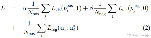
Voxelnet的损失函数与传统的检测任务一样,主要由分类损失和回归损失组成。其中
2.3.2 代码:
    def forward(self, data):
        tag = data[0]                   # len(tag)==5(batch size)
        label = data[1]                 # 5个      表示:标签信息
        vox_feature = data[2]           # list:5   表示:体素特征
        vox_number = data[3]            # list:5   表示:体素数量
        vox_coordinate = data[4]        # list:5   表示:点云坐标

        # group 层
        features = self.feature(vox_feature, vox_number, vox_coordinate)    # [5,10,400,352,128]

        # rpn 层
        prob_output, delta_output = self.rpn(features)                      # [5,2,200,176]  [5,14,200,176]


        # Calculate ground-truth   计算真实的box边框
        # pos_equal_one:[5,200,176,2]
        # neg_equal_one:[5,200,176,2]
        # targets:      [5,200,176,14]
        pos_equal_one, neg_equal_one, targets = cal_rpn_target(label, self.rpn_output_shape, self.anchors, cls = cfg.DETECT_OBJ, coordinate = 'lidar')

        # 注意:沿着最后一个维度重复 7 次,这可能是为了适应目标属性的数量。
        pos_equal_one_for_reg = np.concatenate([np.tile(pos_equal_one[..., [0]], 7), np.tile(pos_equal_one[..., [1]], 7)], axis = -1)   # [5,200,176,14]

        # np.sum(pos_equal_one, axis=(1, 2, 3)) 对 pos_equal_one 在 (height, width, num_classes) 的维度上求和,得到一个形状为 (batch_size,) 的张量。这个结果告诉我们每个批次中每个样本中正样本的数量。
        # reshape(-1, 1, 1, 1) 将求和结果重新形状为 (batch_size, 1, 1, 1) 的张量,这样做主要是为了能够在后续的计算中进行广播(broadcasting),方便和其他张量进行形状匹配或者运算。
        # np.clip(..., a_min=1, a_max=None) 对求和结果进行裁剪操作,确保每个批次中至少有一个正样本。这种操作通常是为了避免出现某些批次没有正样本而导致损失函数计算异常或者无法收敛的情况。
        pos_equal_one_sum = np.clip(np.sum(pos_equal_one, axis = (1, 2, 3)).reshape(-1, 1, 1, 1), a_min = 1, a_max = None)  # [5,1,1,1]
        neg_equal_one_sum = np.clip(np.sum(neg_equal_one, axis = (1, 2, 3)).reshape(-1, 1, 1, 1), a_min = 1, a_max = None)  # [5,1,1,1]

        # Move to gpu
        device = features.device
        pos_equal_one = torch.from_numpy(pos_equal_one).to(device).float()
        neg_equal_one = torch.from_numpy(neg_equal_one).to(device).float()
        targets = torch.from_numpy(targets).to(device).float()
        pos_equal_one_for_reg = torch.from_numpy(pos_equal_one_for_reg).to(device).float()
        pos_equal_one_sum = torch.from_numpy(pos_equal_one_sum).to(device).float()
        neg_equal_one_sum = torch.from_numpy(neg_equal_one_sum).to(device).float()

        # [batch, cfg.FEATURE_HEIGHT, cfg.FEATURE_WIDTH, 2/14] -> [batch, 2/14, cfg.FEATURE_HEIGHT, cfg.FEATURE_WIDTH]
        pos_equal_one = pos_equal_one.permute(0, 3, 1, 2)       # [5,200,176,2]  -> [5,2,200,176]
        neg_equal_one = neg_equal_one.permute(0, 3, 1, 2)       # [5,200,176,2]  -> [5,2,200,176]
        targets = targets.permute(0, 3, 1, 2)                   # [5,200,176,14] -> [5,14,200,176]
        pos_equal_one_for_reg = pos_equal_one_for_reg.permute(0, 3, 1, 2)   # [5,200,176,14] -> [5,14,200,176]

        # Calculate loss    损失函数计算
        cls_pos_loss = (-pos_equal_one * torch.log(prob_output + small_addon_for_BCE)) / pos_equal_one_sum      # [5,2,200,176]
        cls_neg_loss = (-neg_equal_one * torch.log(1 - prob_output + small_addon_for_BCE)) / neg_equal_one_sum  # [5,2,200,176]

        cls_loss = torch.sum(self.alpha * cls_pos_loss + self.beta * cls_neg_loss)
        cls_pos_loss_rec = torch.sum(cls_pos_loss)
        cls_neg_loss_rec = torch.sum(cls_neg_loss)

        reg_loss = smooth_l1(delta_output * pos_equal_one_for_reg, targets * pos_equal_one_for_reg, self.sigma) / pos_equal_one_sum # [5,14,200,176]
        reg_loss = torch.sum(reg_loss)

        loss = cls_loss + reg_loss

        return prob_output, delta_output, loss, cls_loss, reg_loss, cls_pos_loss_rec, cls_neg_loss_rec
总结
1、相比于pointnet系列直接对原始激光点云进行特征提取,voxelnet将原始激光点云进行一个一个voxel的体素化分割,再利用卷积神经网络对体素特征进行特征提取。
2、Voxelnet提出的先体素化再采样的点云特征提取方法大大提高了点云数据的处理速度与精度。
3、Voxelnet的loss计算方案延续了faster R-CNN的RPN结构,借用anchors先验眶,对Feature network提出的特征进行处理,使用 cls-head 和 reg-head 进行 类别置信度 和 回归 bounding box的计算
参考
点云学习笔记11——VoxelNet算法+代码运行_voxel-net代码运行环境 csdn-CSDN博客
代码复现: VoxelNet论文和代码解析 pytorch版本_voxelnet pytorch 跑通-CSDN博客
无人驾驶汽车系统入门(二十八)——基于VoxelNet的激光雷达点云车辆检测及ROS实现_基于3d-voxel的无人驾驶场景点云目标检测和分割-CSDN博客
Faster RCNN原理篇(三)——区域候选网络RPN(Region Proposal Network)的学习、理解-CSDN博客