import pandas as pd
import numpy as np
import matplotlib.pyplot as plt
import sys
import scipy.io
import scipy.signal as signal
from skimage.restoration import denoise_wavelet
from scipy.interpolate import interp1d
import colorednoise as cn
%matplotlib inline
#pip install xlrd
df = pd.read_excel('frequency.xls')
df.head()| Timestamp | BADARPUR:Frequency | |
| 0 | 2021-09-11 06:12:16.840 | 50.008 |
| 1 | 2021-09-11 06:12:16.880 | 50.008 |
| 2 | 2021-09-11 06:12:16.920 | 50.009 |
| 3 | 2021-09-11 06:12:16.960 | 50.009 |
| 4 | 2021-09-11 06:12:17.000 | 50.008 |
df['BADARPUR:Frequency']
0        50.008
1        50.008
2        50.009
3        50.009
4        50.008
          ...
65530    49.981
65531    49.982
65532    49.982
65533    49.982
65534    49.982
Name: BADARPUR:Frequency, Length: 65535, dtype: float64
def calculate_psnr(signalnal, distorted_signal):
    # Ensure the signals have the same shape and data type
    # signalnal = signalnal.astype(np.float64)
    # distorted_signal = distorted_signal.astype(np.float64)


    # Calculate the mean squared error (MSE)
    mse = np.mean((signalnal - distorted_signal) ** 2)


    # Calculate the maximum possible power of the original signal
    max_power = np.max(signalnal) ** 2


    # Calculate the PSNR using the formula
    psnr = 10 * np.log10(max_power / mse)


    return psnr
import numpy as np
from skimage.metrics import structural_similarity as ssim


def calculate_ssim(image1, image2):
    # Calculate the SSIM
    ssim_value = ssim(image1, image2, multichannel=False)


    return ssim_value


def find_params(reconstructed_signal, signal):
    print("snr of the signal needed is: ", 20*np.log10(reconstructed_signal.mean()/reconstructed_signal.std()))
    print("snr of the original signal is: ", 20*np.log10(signal.mean()/signal.std()))
    print('peaksnr of the signal needed is: ', calculate_psnr(signal, reconstructed_signal))
    print('Structure similarity index', calculate_ssim(signal, reconstructed_signal))
    print("Mean of reconstructed_signal: ", np.mean(reconstructed_signal))
    print("Median of reconstructed_signal: ", np.median(reconstructed_signal))
    print("Variance of reconstructed_signal: ", np.var(reconstructed_signal))
    print("Standard deviation of reconstructed_signal: ", np.std(reconstructed_signal))
    print('Correlation between original and reconstructed_signal: ', np.corrcoef(reconstructed_signal, signal)[0,1])
    print('frequency content/range of noise: ',np.abs(signal-reconstructed_signal).max())
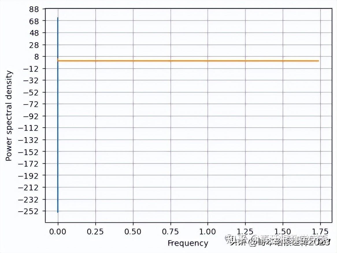
# psd, skewness, kurtosis


def kaveri(t, signal):
    print(f'Kurtosis : {scipy.stats.kurtosis(signal)}')
    print(f'Skewness : {scipy.stats.skew(signal)}')


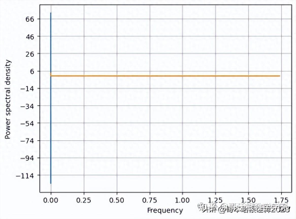
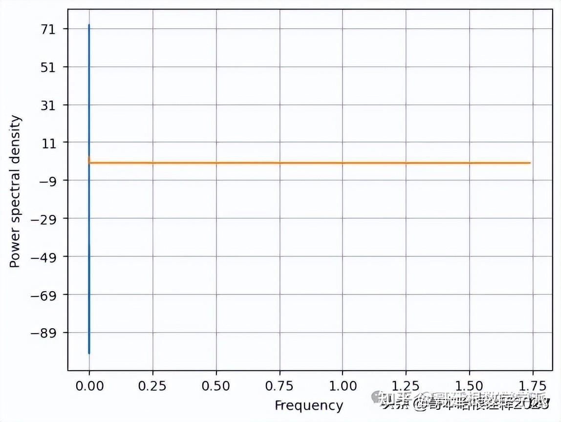
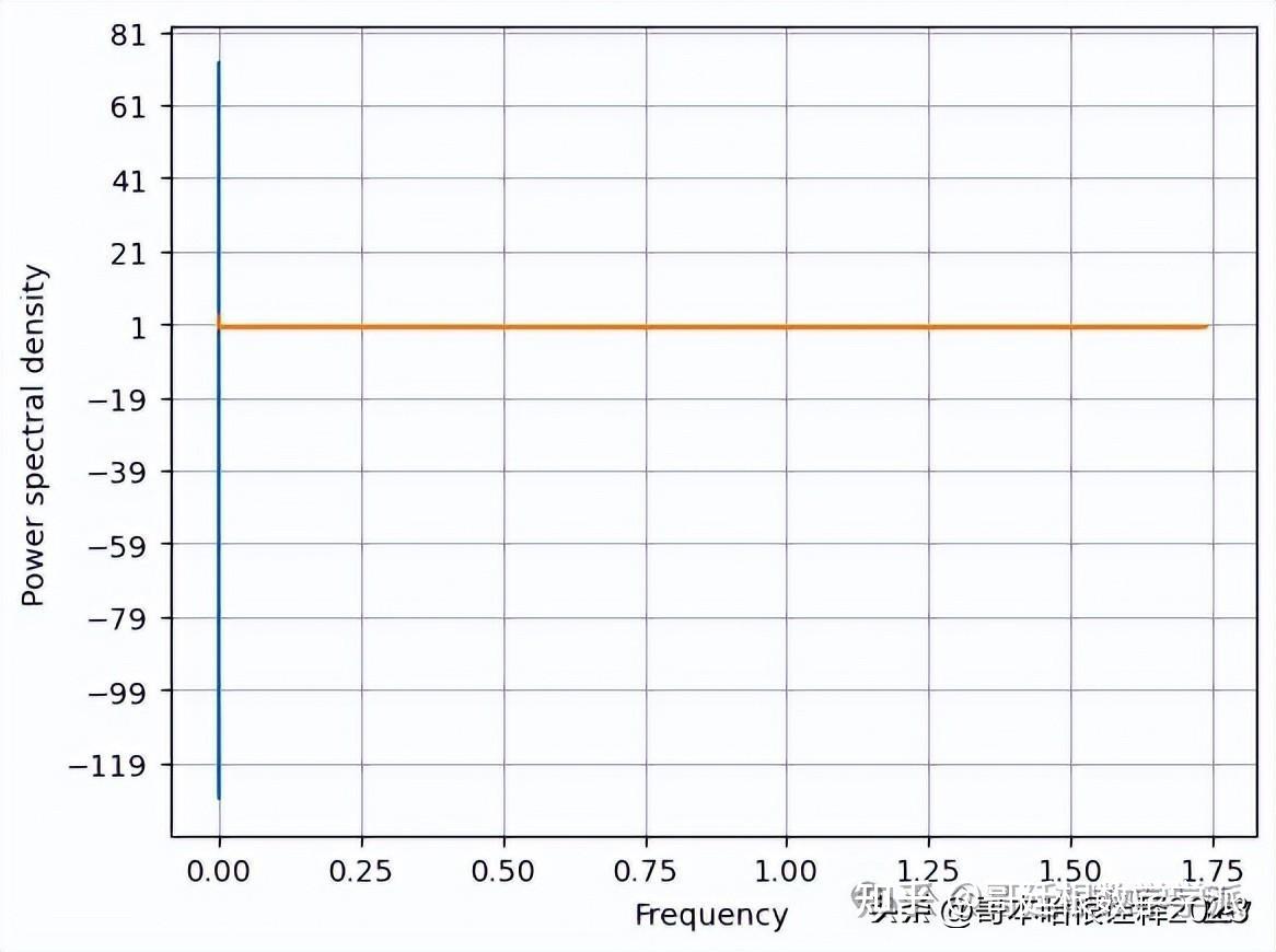
    f, Pxx_den = plt.psd(signal, NFFT=len(t), Fs=2*np.pi)


    # Plot the PSD
    plt.plot(f, Pxx_den)
    plt.xlabel('Frequency')
    plt.ylabel('Power spectral density')
    plt.show()


# Section of filters


def EMD(x):
    # Define stopping criterion
    MAXITER = 100
    TOLERANCE = 0.001

    # Initialize variables
    h = x
    d = np.zeros_like(x)
    n = 1

    # Loop until stopping criterion is met
    while n < MAXITER and np.abs(h).sum() > TOLERANCE:
        # Compute mean of envelope
        m = signal.hilbert(h).imag

        # Subtract mean from signal
        d += h - m

        # Update residual
        h = m

        # Increment iteration counter
        n += 1

    # Return IMF components and residual
    return d, h


def median_filter(signal, window_size = 10):
    """
    Applies a median filter to a signal to remove noise.
    Inputs:
        signal: numpy array containing the signal
        window_size: size of the window used for the filter
    Returns:
        filtered_signal: numpy array containing the filtered signal
    """
    # Pad the signal to handle edges
    signal_padded = np.pad(signal, int(window_size/2), mode='reflect')

    # Initialize the filtered signal
    filtered_signal = np.zeros_like(signal)

    # Loop through the signal and apply the median filter
    for i in range(len(signal)):
        window = signal_padded[i:i+window_size]
        filtered_signal[i] = np.median(window)

    return filtered_signal


def triangular_filter(signal, window_size):
    """
    Applies a moving average triangular filter to a signal to smooth it out.
    Inputs:
        signal: numpy array containing the signal
        window_size: size of the window used for the filter
    Returns:
        filtered_signal: numpy array containing the filtered signal
    """
    # Create a triangular window
    window = np.array(list(range(1, window_size//2+1)) + [window_size//2+1] + list(range(window_size//2, 0, -1)), dtype=np.float32)

    # Normalize the window
    window /= np.sum(window)

    # Apply the filter to the signal using convolution
    filtered_signal = np.convolve(signal, window, mode='same')

    return filtered_signal


def wavelet_filter(signal):
    """
    Applies a wavelet filter to a signal to remove noise.
    Inputs:
        signal: numpy array containing the signal
    Returns:
        filtered_signal: numpy array containing the filtered signal
    """
    # Apply the filter
    filtered_signal = denoise_wavelet(signal, method='BayesShrink', mode='soft', wavelet_levels=3, wavelet='db4', rescale_sigma=True)

    return filtered_signal


def eidft_clean(signal, sampling_rate, noise_std_dev):
    """
    Cleans noise from a signal using Enhanced Interpolated Discrete Fourier Transform.
    Inputs:
        signal: numpy array containing the noisy signal
        sampling_rate: sampling rate of the signal
        noise_std_dev: standard deviation of the noise
    Returns:
        cleaned_signal: numpy array containing the cleaned signal
    """
    # Compute the DFT of the noisy signal
    X = np.fft.fft(signal)

    # Compute the frequency-domain filter
    N = len(signal)
    f = np.arange(N) * sampling_rate / N
    filter = np.exp(-((2*np.pi*f)**2) / (2*(noise_std_dev**2)))

    # Apply the frequency-domain filter to the DFT of the signal
    X_filtered = X * filter

    # Compute the cleaned signal using the inverse DFT
    cleaned_signal = np.fft.ifft(X_filtered).real

    # Interpolate the cleaned signal to the original sampling rate
    t = np.arange(len(cleaned_signal))
    interp_func = interp1d(t, cleaned_signal, kind='cubic')
    t_interp = np.linspace(0, N-1, N) * (1/sampling_rate)
    filtered_signal = interp_func(t_interp)

    return filtered_signal


def extended_kalman_filter(signal, sampling_rate, noise_std_dev):
    """
    Cleans noise from a signal using Extended Kalman Filter.
    Inputs:
        signal: numpy array containing the noisy signal
        sampling_rate: sampling rate of the signal
        noise_std_dev: standard deviation of the noise
    Returns:
        cleaned_signal: numpy array containing the cleaned signal
    """
    # Define the state transition matrix
    A = np.array([[1, 1/sampling_rate], [0, 1]])

    # Define the observation matrix
    H = np.array([[1, 0]])

    # Define the process noise covariance matrix
    Q = np.array([[1, 0], [0, 1]])

    # Define the observation noise covariance matrix
    R = np.array([[noise_std_dev**2]])

    # Define the initial state estimate
    x = np.array([[signal[0]], [0]])

    # Define the initial error covariance matrix
    P = np.array([[1, 0], [0, 1]])

    # Initialize the cleaned signal
    filtered_signal = np.zeros_like(signal)

    # Loop through the signal and apply the Kalman filter
    for i in range(len(signal)):
        # Predict the next state
        x = A @ x

        # Predict the next error covariance matrix
        P = A @ P @ A.T + Q

        # Compute the Kalman gain
        K = P @ H.T @ np.linalg.inv(H @ P @ H.T + R)

        # Update the state estimate
        x = x + K @ (signal[i] - H @ x)

        # Update the error covariance matrix
        P = (np.eye(2) - K @ H) @ P

        # Save the cleaned signal
        filtered_signal[i] = x[0, 0]

    return filtered_signal


# Section of plots


def plot(t, signal, title, alpha=1):
    plt.figure(figsize=(20,8))
    plt.title(f'{signal}')
    plt.plot(t, signal, alpha=alpha)
    plt.xlabel('Time')
    plt.ylabel('Amplitude')
    plt.title(f'{title} analysis')
    if plt.gca().get_legend():
        plt.legend()


# Section of signal parameter analysis


def snr(filtered_signal):
    snr1 = 20*np.log10(filtered_signal.mean()/filtered_signal.std())
    print(f'snr: {snr1}')


def nrmse(filtered_signal):
    print(f"nrmse: {filtered_signal.std()/filtered_signal.mean()}")


def tve(filtered_signal, noisy_signal):
    print(f"tve: {np.linalg.norm((filtered_signal-noisy_signal)/noisy_signal)}")


def cr(filtered_signal, noisy_signal):
    print(f"cr: {np.ptp(filtered_signal)/np.ptp(noisy_signal)}")


def signal_params(filtered_signal, noisy_signal):
    return snr(filtered_signal), nrmse(filtered_signal), tve(filtered_signal, noisy_signal), cr(filtered_signal, noisy_signal)


# automation


def automate(title, signal, reconstructed_signal, noisy_signal, t):
    # Plot results
    title = title
    print(title)
    plot(t, reconstructed_signal, title=title)
    plt.plot(t, noisy_signal)
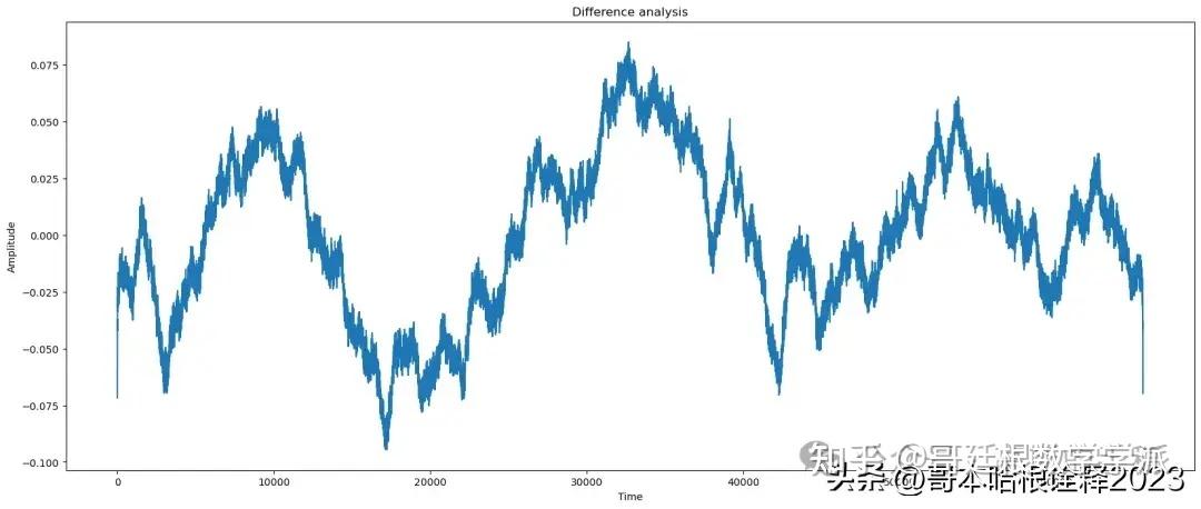
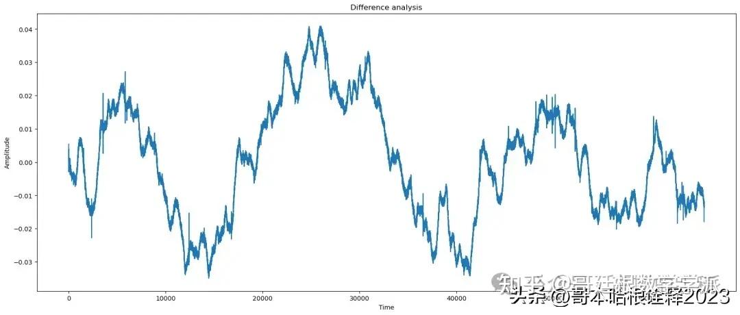
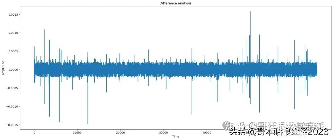
    title = 'Difference'
    plot(t, signal - reconstructed_signal, title=title)


    signal_params(reconstructed_signal, noisy_signal)
    plt.figure()
    kaveri(t, reconstructed_signal)


# actual function


def signal_analysis(signal, var = 0.003, noise_type = ['white', 'pink', '0.1 inc white', '0.1 inc pink', '0.1 dec white', '0.1 dec pink']):
    t = np.arange(0,signal.shape[0],1)


    print(f'Original signal analysis: ')
    kaveri(t, signal);
    find_params(signal, signal)
    signal_params(signal, signal)
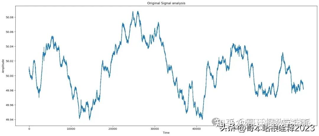
    plot(t,signal, title = 'Original Signal');


    # Generate noisy signal
    if noise_type == 'white':
        n =  np.random.rand(signal.shape[0])
        noise = ((n - n.mean())/n.std())*var

    elif noise_type == 'pink':
        n = cn.powerlaw_psd_gaussian(1, signal.shape[0])
        noise = ((n - n.mean())/n.std())*var

    elif noise_type == '0.1 inc white':
        n =  np.random.rand(signal.shape[0])
        noise = ((n - n.mean())/n.std())*var
        noise = noise + 0.1*noise

    elif noise_type == '0.1 inc pink':
        n = cn.powerlaw_psd_gaussian(1, signal.shape[0])
        noise = ((n - n.mean())/n.std())*var
        noise = noise + 0.1*noise

    elif noise_type == '0.1 dec white':
        n =  np.random.rand(signal.shape[0])
        noise = ((n - n.mean())/n.std())*var
        noise = noise - 0.1*noise

    elif noise_type == '0.1 dec pink':
        n = cn.powerlaw_psd_gaussian(1, signal.shape[0])
        noise = ((n - n.mean())/n.std())*var
        noise = noise - 0.1*noise


    noisy_signal = signal + noise
    print(f'Noisy signal analysis: ');
    find_params(noisy_signal, signal)
    signal_params(noisy_signal, signal)
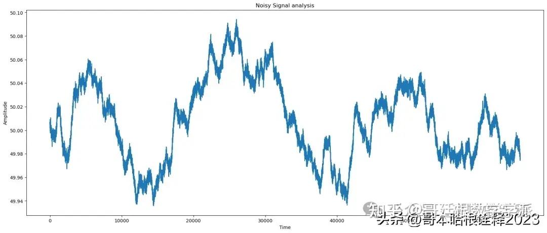
    plot(t,noisy_signal, title='Noisy Signal');


    print(f"EMD Analysis of signal")


    # Apply EMD
    IMFs = []
    residual = noisy_signal
    for i in range(10):
        imf, residual = EMD(residual)
        IMFs.append(imf)

    # Reconstruct signal using selected IMFs
    reconstructed_signal = np.sum(IMFs[:3], axis=0)


    find_params(reconstructed_signal, signal)


    # Plot results
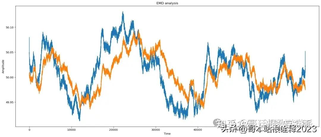
    automate("EMD", signal, reconstructed_signal, noisy_signal, t)

    # apply Median


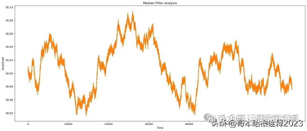
    reconstructed_signal = median_filter(noisy_signal, window_size = 10)


    # median analysis
    print(f"Median Analysis of signal")
    find_params(reconstructed_signal, signal)
    automate('Median Filter',signal, reconstructed_signal, noisy_signal, t)

    # apply Triangular
    reconstructed_signal = triangular_filter(noisy_signal, window_size = 10)


    # triangular analysis
    print(f"Triangular Analysis of signal")
    find_params(reconstructed_signal, signal)
    automate('Triangular Filter',signal, reconstructed_signal, noisy_signal, t)


    # apply Wavelet
    reconstructed_signal = wavelet_filter(noisy_signal)


    # wavelet analysis
    print(f"Wavelet Analysis of signal")
    find_params(reconstructed_signal, signal)
    automate('Wavelet Filter',signal, reconstructed_signal, noisy_signal, t)

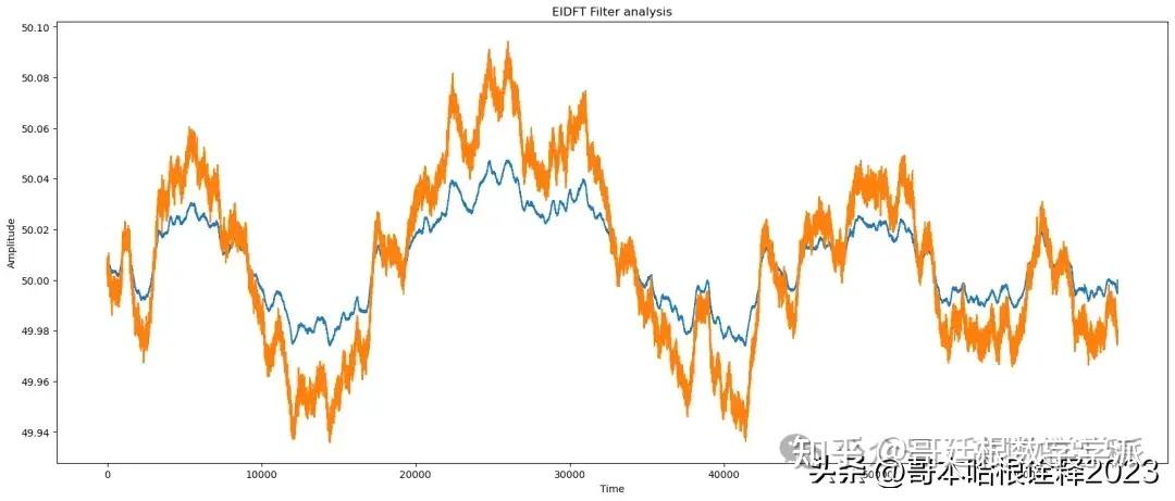
    # apply EIDFT
    reconstructed_signal = eidft_clean(signal, sampling_rate =1, noise_std_dev = 0.5)


    # eidft analysis
    print(f"EIDFT Analysis of signal")
    find_params(reconstructed_signal, signal)
    automate('EIDFT Filter',signal, reconstructed_signal, noisy_signal, t)


    # apply EKF
    reconstructed_signal = extended_kalman_filter(signal, sampling_rate =1, noise_std_dev = 0.5)


    # ekf analysis
    print(f"EKF Analysis of signal")
    find_params(reconstructed_signal, signal)
    automate('EKF Filter',signal, reconstructed_signal, noisy_signal, t)
signal_analysis(df['BADARPUR:Frequency'], noise_type='0.1 inc pink')
Original signal analysis:
Kurtosis : -0.7962090526109451
Skewness : 0.13436966529721817
snr of the signal needed is: 63.359398370474736
snr of the original signal is: 63.359398370474736
peaksnr of the signal needed is: inf
Structure similarity index 1.0
Mean of reconstructed_signal: 50.00740880445562
Median of reconstructed_signal: 50.008
Variance of reconstructed_signal: 0.001153777961697126
Standard deviation of reconstructed_signal: 0.0339673072482516
Correlation between original and reconstructed_signal: 0.9999999999999998
frequency content/range of noise: 0.0
snr: 63.359398370474736
nrmse: 0.0006792506793940005
tve: 0.0
cr: 1.0
Noisy signal analysis:
snr of the signal needed is: 63.372344969998124
snr of the original signal is: 63.359398370474736
peaksnr of the signal needed is: 83.62439501798347
Structure similarity index 0.9993235421201816
Mean of reconstructed_signal: 50.007408804455636
Median of reconstructed_signal: 50.007793103186636
Variance of reconstructed_signal: 0.0011503435965118651
Standard deviation of reconstructed_signal: 0.03391671559145822
Correlation between original and reconstructed_signal: 0.9952747924519362
frequency content/range of noise: 0.015217348031306699
snr: 63.372344969998124
nrmse: 0.0006782389884466603
tve: 0.016894424454212655
cr: 1.0642173110539879
EMD Analysis of signal
snr of the signal needed is: 60.36211128295382
snr of the original signal is: 63.359398370474736
peaksnr of the signal needed is: 63.273718891916964
Structure similarity index 0.9985459269801901
Mean of reconstructed_signal: 50.007408804455636
Median of reconstructed_signal: 50.00830343318955
Variance of reconstructed_signal: 0.002300687193023832
Standard deviation of reconstructed_signal: 0.04796547918059229
Correlation between original and reconstructed_signal: 0.6978283142117662
frequency content/range of noise: 0.09464395825857252
EMD
snr: 60.36211128295382
nrmse: 0.0009591674579291256
tve: 0.17362096944802632
cr: 1.3843324411761402
Kurtosis : -0.8722024163896163
Skewness : 0.16467170432487924Median Analysis of signal
snr of the signal needed is: 63.38318616124973
snr of the original signal is: 63.359398370474736
peaksnr of the signal needed is: 84.49955024940508
Structure similarity index 0.9998265854178908
Mean of reconstructed_signal: 50.00740788778814
Median of reconstructed_signal: 50.008025452121394
Variance of reconstructed_signal: 0.0011474930694798963
Standard deviation of reconstructed_signal: 0.03387466707555804
Correlation between original and reconstructed_signal: 0.9961351976024705
frequency content/range of noise: 0.014740105840992612
Median Filter
snr: 63.38318616124973
nrmse: 0.0006773929804874024
tve: 0.007950599595301146
cr: 0.957195800692995
Kurtosis : -0.84887960677991
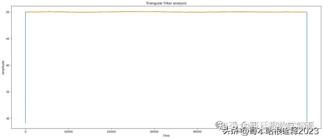
Skewness : 0.14449305288134331Triangular Analysis of signal
snr of the signal needed is: 50.35798720799019
snr of the original signal is: 63.359398370474736
peaksnr of the signal needed is: 50.599316568347454
Structure similarity index 0.9996881092897941
Mean of reconstructed_signal: 50.00592686239261
Median of reconstructed_signal: 50.00801458877254
Variance of reconstructed_signal: 0.023027364842180365
Standard deviation of reconstructed_signal: 0.15174770127478163
Correlation between original and reconstructed_signal: 0.22593033630499942
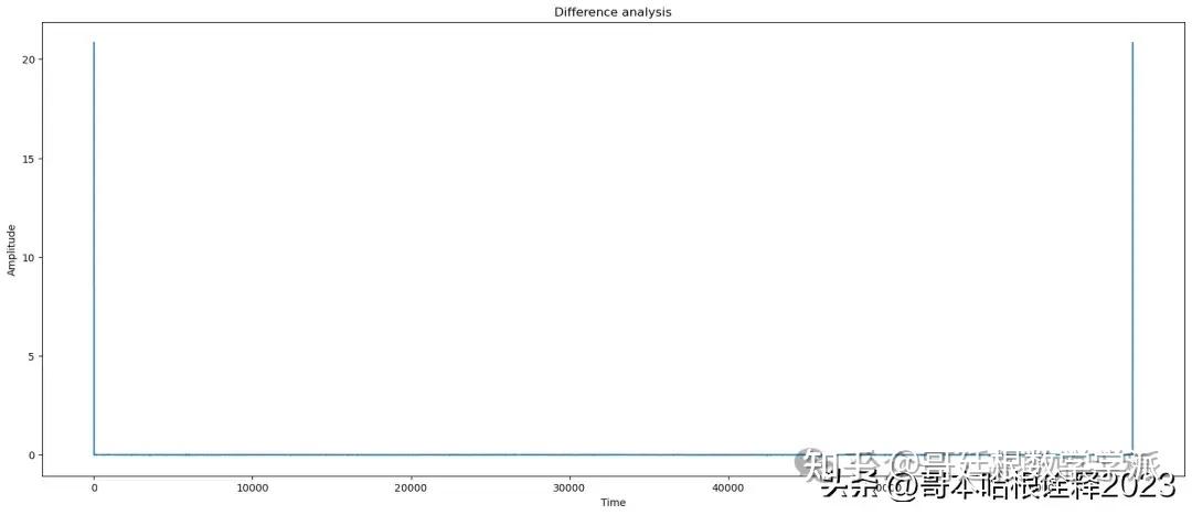
frequency content/range of noise: 20.838068518161432
Triangular Filter
snr: 50.35798720799019
nrmse: 0.003034594313037417
tve: 0.7566914641337033
cr: 132.03832044932048
Kurtosis : 13308.859735828964
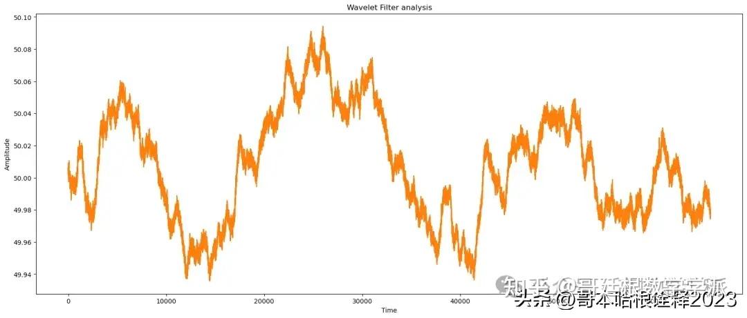
Skewness : -108.29963633991207Wavelet Analysis of signal
snr of the signal needed is: 63.37914279440283
snr of the original signal is: 63.359398370474736
peaksnr of the signal needed is: 84.19070197067637
Structure similarity index 0.9997166942858678
Mean of reconstructed_signal: 50.00740882209381
Median of reconstructed_signal: 50.00795045174669
Variance of reconstructed_signal: 0.001148561948438932
Standard deviation of reconstructed_signal: 0.03389044036950438
Correlation between original and reconstructed_signal: 0.9958508386593179
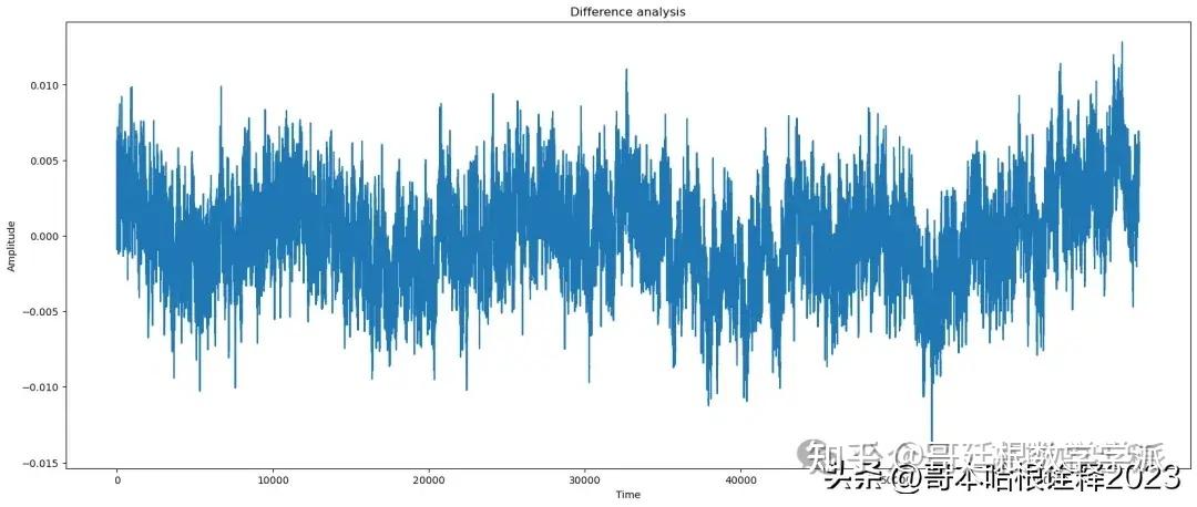
frequency content/range of noise: 0.014050147282368641
Wavelet Filter
snr: 63.37914279440283
nrmse: 0.0006777083869726763
tve: 0.00570299520742053
cr: 0.9784526863900248
Kurtosis : -0.8475890499793493
Skewness : 0.1442894763680122EIDFT Analysis of signal
snr of the signal needed is: 69.38127515487265
snr of the original signal is: 63.359398370474736
peaksnr of the signal needed is: 69.39093712514465
Structure similarity index 0.9999139278707353
Mean of reconstructed_signal: 50.007408804455636
Median of reconstructed_signal: 50.007871931762196
Variance of reconstructed_signal: 0.0002883640973523934
Standard deviation of reconstructed_signal: 0.016981286681296955
Correlation between original and reconstructed_signal: 0.999890339844553
frequency content/range of noise: 0.04091477862992576
EIDFT Filter
snr: 69.38127515487265
nrmse: 0.0003395754166687383
tve: 0.08752573053472566
cr: 0.4637084486960638
Kurtosis : -0.79658651249113
Skewness : 0.1344308232670232EKF Analysis of signal
snr of the signal needed is: 63.35962997195324
snr of the original signal is: 63.359398370474736
peaksnr of the signal needed is: 116.4119741610082
Structure similarity index 0.99999816134827
Mean of reconstructed_signal: 50.00740880442131
Median of reconstructed_signal: 50.00807517919881
Variance of reconstructed_signal: 0.0011537340392742852
Standard deviation of reconstructed_signal: 0.03396666070243416
Correlation between original and reconstructed_signal: 0.9999975163275431
frequency content/range of noise: 0.0015751073696321782
EKF Filter
snr: 63.35962997195324
nrmse: 0.0006792325680236218
tve: 0.01689813054863477
cr: 0.938414454803866
Kurtosis : -0.7962683996090929学术咨询:
担任《Mechanical System and Signal Processing》《中国电机工程学报》等期刊审稿专家,擅长领域:信号滤波/降噪,机器学习/深度学习,时间序列预分析/预测,设备故障诊断/缺陷检测/异常检测。
分割线分割线分割线分割线分割线分割线
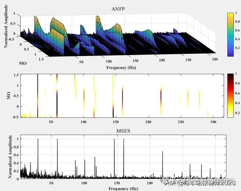
一种基于非线性滤波过程的旋转机械故障诊断方法(MATLAB)
该非线性滤波方法对旋转机械振动信号进行傅里叶变换获得频域幅值谱和相位谱,通过对其幅值谱赋予不同权重的指数,并结合原始信号相位谱进行逆傅里叶变换,从而获得一系列的修正信号,最后通过修正信号平方包络的功率谱识别故障特征.
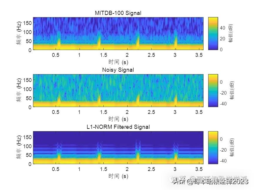
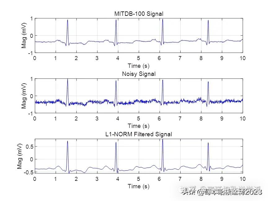
基于L1范数惩罚的稀疏正则化最小二乘心电信号降噪方法(Matlab R2021B)
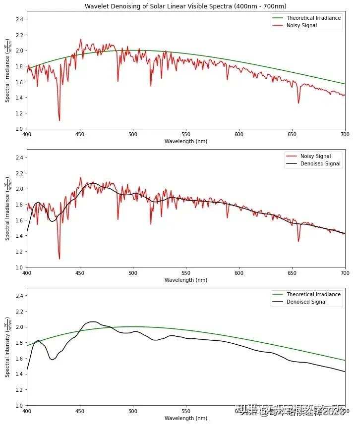
基于小波分析的Linear电磁谱降噪(Python)
Python环境下基于最小最大凹面全变分一维信号降噪方法

